Prediction

POL51

Juan Tellez

jftellez@ucdavis.edu

UC Davis

October 28, 2024

Plan for today

Making predictions

Multiple regression

How right are we?

Why predict?

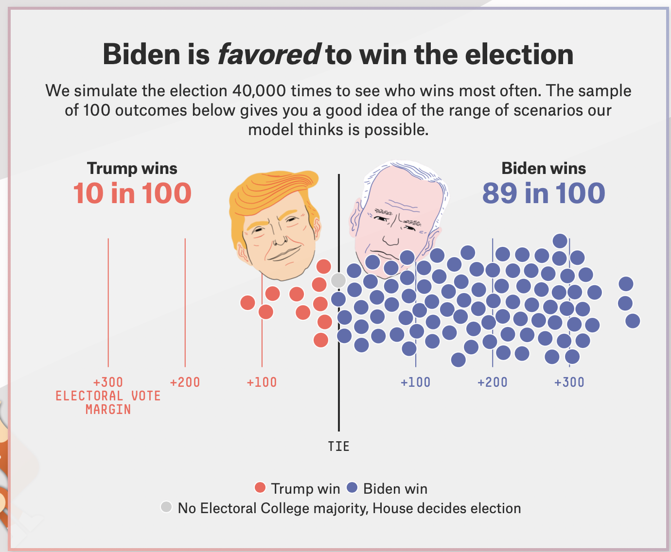
Companies, policymakers, and academics want to predict
who will win an election
whether UN peacekeepers can reduce conflict
whether you’ll get the vaccine or not
At stake is what decision to take under uncertainty about the future

Making predictions

The basics of prediction are pretty straightforward:

Take/collect existing data ✅
Fit a model to it ✅
Design a scenario you want a prediction for ☑️
Use the model to generate an estimate for that scenario ☑️

What’s the scenario?

A scenario is a hypothetical observation (real, or imagined) that we want a prediction for
You define a scenario by picking values for explanatory variables
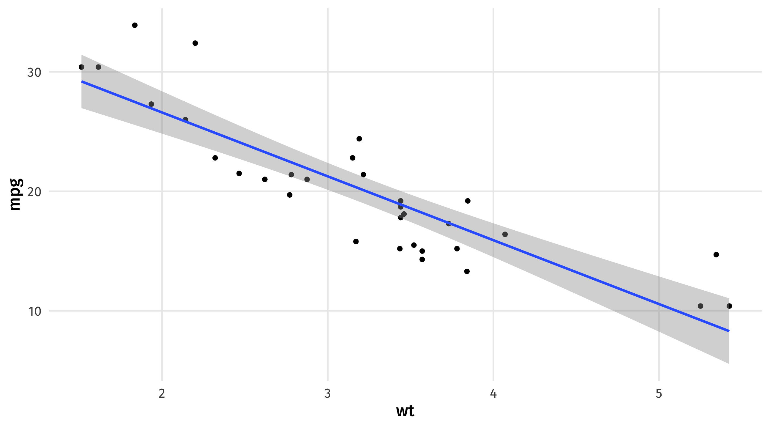
Example: what is the predicted fuel efficiency for a car that weighs 3.25 tons?

Prediction (by hand)

weight_model = lm(mpg ~ wt, data = mtcars)

Remeber our model is an equation:

$\widehat{mpg} = 37.29 - 5.34(wt)$

Scenario: a car that weights 3.25 tons $\rightarrow$ what fuel efficiency should we expect?

To get an estimate of mpg, we simply plug in the value of “weight” we are interested in:

$\widehat{mpg} = 37.29 - 5.34 \times \color{red}{3.25} = 19.935$

Prediction (in R)

First define the scenario we want a prediction for, using crossing()

weight_scenario = crossing(wt = 3.25) 
weight_scenario

# A tibble: 1 × 1
     wt
  <dbl>
1  3.25

Note that I store this as a data object

Note

the variables in crossing have to have the same name as the variables in the model

Prediction (in R)

We can then combine our scenario with our model using augment()

augment(weight_model, newdata = weight_scenario)

# A tibble: 1 × 2
     wt .fitted
  <dbl>   <dbl>
1  3.25    19.9

augment plugs in scenario to our model to get an estimate

Note we got the same answer as when we did it by hand

Note

We tell augment what our new scenario is using the newdata = argument

Multiple scenarios

We can also look at multiple scenarios: a light, medium, and heavy car:

weight_scenario = crossing(wt = c(1.5, 3, 5)) 
weight_scenario

# A tibble: 3 × 1
     wt
  <dbl>
1   1.5
2   3  
3   5

And then use augment to get the estimates:

augment(weight_model, newdata = weight_scenario)

# A tibble: 3 × 2
     wt .fitted
  <dbl>   <dbl>
1   1.5    29.3
2   3      21.3
3   5      10.6

Sequence of scenarios

Or we can look at a sequence of scenarios using the seq() function

Example: every weight between 2 and 6 tons, in .1 ton increments

seq_weights = crossing(wt = seq(from = 2, to = 6, by = .1)) 
seq_weights

# A tibble: 41 × 1
      wt
   <dbl>
 1   2  
 2   2.1
 3   2.2
 4   2.3
 5   2.4
 6   2.5
 7   2.6
 8   2.7
 9   2.8
10   2.9
# ℹ 31 more rows

Note

seq needs a starting point (from), an end point (to), and an interval (by)

Prediction (in R)

And then get predictions for all these scenarios:

weight_preds = augment(weight_model, newdata = seq_weights)
weight_preds

# A tibble: 41 × 2
      wt .fitted
   <dbl>   <dbl>
 1   2      26.6
 2   2.1    26.1
 3   2.2    25.5
 4   2.3    25.0
 5   2.4    24.5
 6   2.5    23.9
 7   2.6    23.4
 8   2.7    22.9
 9   2.8    22.3
10   2.9    21.8
# ℹ 31 more rows

Trivial

Do we really need a model to predict MPG when weight = 3.25? Probably not

Multiple regression

The real power of modeling and prediction comes with using multiple explanatory variables

Many factors influence a car’s fuel efficiency; we can use that information to make more precise predictions

	mpg	wt	cyl	hp	am	vs
Mazda RX4	21.0	2.62	6	110	1	0
Merc 280C	17.8	3.44	6	123	0	1
Pontiac Firebird	19.2	3.85	8	175	0	0
Mazda RX4 Wag	21.0	2.88	6	110	1	0

Multiple regression

Here, a car’s fuel efficiency is a function of its weight (wt), number of cylinders (cyl), horse power (hp), and whether its transmission is manual or automatic (am)

big_model = lm(mpg ~ wt + cyl + hp + am, data = mtcars)

The model equation we want in the end is this one:

\[\operatorname{mpg} = \beta_0 + \color{red}{\beta_{1}}(\operatorname{wt}) + \color{red}{\beta_{2}}(\operatorname{cyl}) + \color{red}{\beta_{3}}(\operatorname{hp}) + \color{red}{\beta_{4}}(\operatorname{am})\]

Multiple regression

Just as when we had one variable, our OLS model is trying to find the values of $\beta$ that “best” fits the data
OLS estimator = $\sum{(Y_i - \hat{Y_i})^2}$
Where $\widehat{Y} = \beta_0 + \beta_1 x_1 + . . . \beta_4 x_4$
Now searching for $\beta_0 ... \beta_4$ to minimize loss function

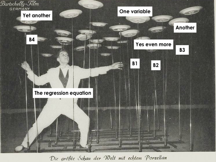
lm() hard at work

Interpretation

term	estimate
(Intercept)	36.15
wt	-2.61
cyl	-0.75
hp	-0.02
am	1.48

wt = every ton of weight is associated with a 2.61 decrease in mpg
cyl = every cylinder is associated with a .7 decrease in mpg
hp = every unit of horse power is associated with a .02 decrease in mpg
am = on average, cars with manual transmissions (am = 1) have 1.48 more mpg than cars with automatic transmissions (am = 0)

Prediction (by hand)

We can make predictions just as before, plugging in values for our explanatory variables

\[ \operatorname{\widehat{mpg}} = 36.15 - 2.61(\operatorname{wt}) - 0.75(\operatorname{cyl}) - 0.02(\operatorname{hp}) + 1.48(\operatorname{am}) \]

With more variables, we can create more specific scenarios

For example: a car that weighs 3 tons, has 4 cylinders, 120 horsepower, and has a manual transmission

\[ \operatorname{\widehat{mpg}} = 36.15 - 2.61 \times \color{blue}{3} - 0.75 \times \color{blue}{4} - 0.02 \times \color{blue}{120} + 1.48 \times \color{blue}{1} \]

\[ \operatorname{\widehat{mpg}} = 24 \]

Prediction (in R)

We can do this in R with crossing() and augment()

big_scenario = crossing(wt = 3, cyl = 4, hp = 120, am = 1)

augment(big_model, newdata = big_scenario)

# A tibble: 1 × 5
     wt   cyl    hp    am .fitted
  <dbl> <dbl> <dbl> <dbl>   <dbl>
1     3     4   120     1    23.8

Troubleshooting

Note that your scenario needs to include every variable in your model, otherwise you will get an error

The one below is missing cylinders, which is in big_model, and won’t run:

bad_scenario = crossing(wt = 3, hp = 120, am = 1)

augment(big_model, newdata = bad_scenario)

Pick scenarios that make sense

Note that to make predictions that make sense, we have to look through our data and see what values are plausible for the variables

For example, a scenario where we set am = 3 doesn’t make sense, since am is a dummy variable that takes two values (0 = automatic, 1 = manual)

But R doesn’t know that, and will give you (nonsensical) estimates:

crazy_car = crossing(wt = 3, cyl = 4, hp = 120, am = 3)
augment(big_model, newdata = crazy_car)

# A tibble: 1 × 5
     wt   cyl    hp    am .fitted
  <dbl> <dbl> <dbl> <dbl>   <dbl>
1     3     4   120     3    26.8

Note

Remember data |> distinct(variable) to see a variable’s values

Holding all else constant

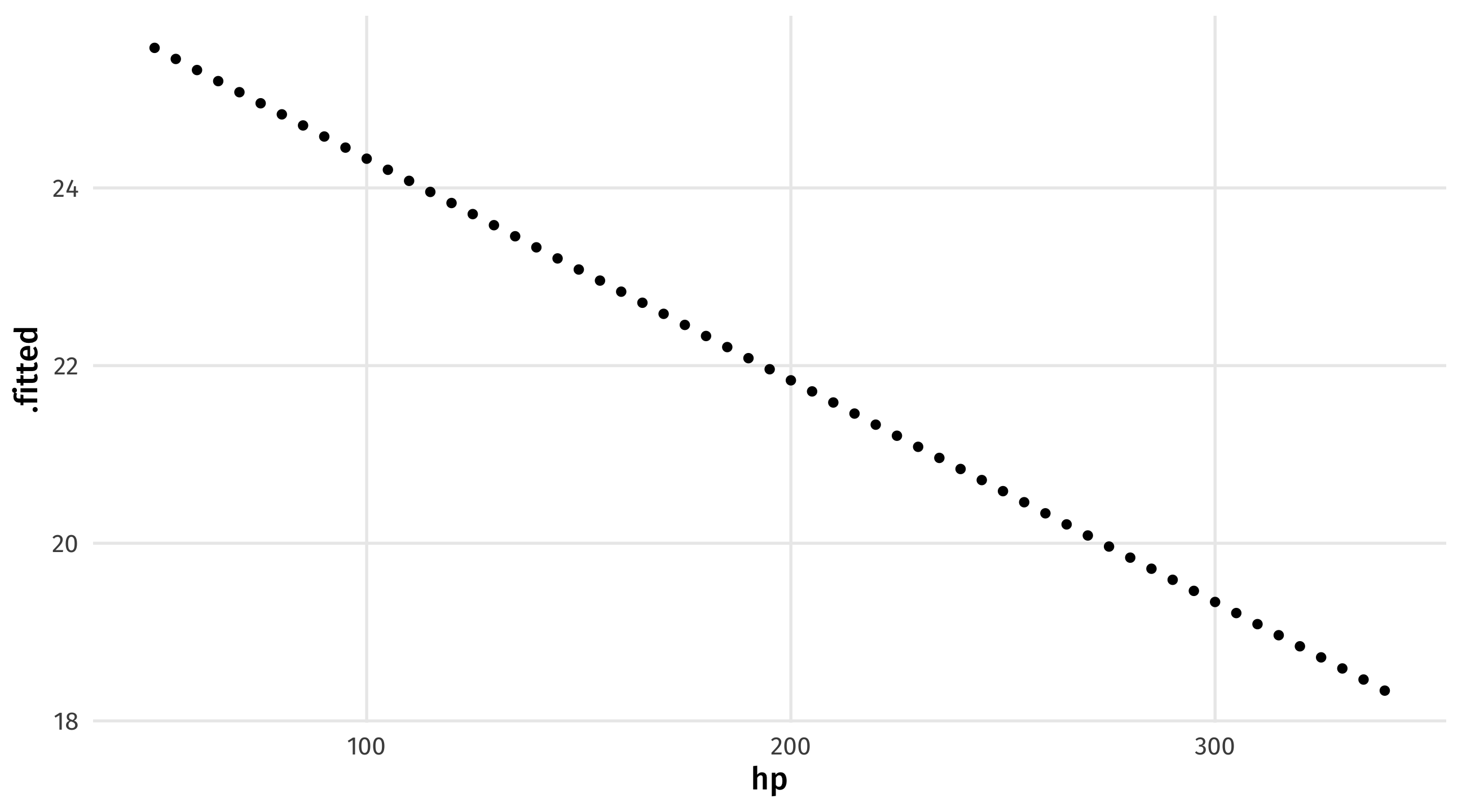
One cool part of multiple regression is that we can see what happens to our estimates when one variable changes but the others are held at a fixed value

Holding all else in the model constant, how does increasing a car’s horsepower change its fuel efficiency?

Holding all else constant

We can use seq() to see what happens when horsepower changes while everything else is left at a fixed value

varying_hp = crossing(wt = 3, cyl = 4, am = 1, hp = seq(from = 50, to = 340, by = 5))

augment(big_model, newdata = varying_hp)

# A tibble: 59 × 5
      wt   cyl    am    hp .fitted
   <dbl> <dbl> <dbl> <dbl>   <dbl>
 1     3     4     1    50    25.6
 2     3     4     1    55    25.5
 3     3     4     1    60    25.3
 4     3     4     1    65    25.2
 5     3     4     1    70    25.1
 6     3     4     1    75    25.0
 7     3     4     1    80    24.8
 8     3     4     1    85    24.7
 9     3     4     1    90    24.6
10     3     4     1    95    24.5
# ℹ 49 more rows

Visualizing predictions

We could then store our estimate, and use it for plotting

hp_pred = augment(big_model, newdata = varying_hp)
ggplot(hp_pred, aes(x = hp, y = .fitted)) + geom_point()

One more example: Gapminder

Say we wanted to predict a country’s life expectancy, using population, GDP per capita, the year, and what continent it is in:

life_model = lm(lifeExp ~ gdpPercap + pop + year + continent, data = gapminder)
tidy(life_model)

# A tibble: 8 × 5
  term              estimate std.error statistic   p.value
  <chr>                <dbl>     <dbl>     <dbl>     <dbl>
1 (Intercept)       -5.18e+2   1.99e+1    -26.1  3.25e-126
2 gdpPercap          2.98e-4   2.00e-5     14.9  2.52e- 47
3 pop                1.79e-9   1.63e-9      1.10 2.73e-  1
4 year               2.86e-1   1.01e-2     28.5  4.80e-146
5 continentAmericas  1.43e+1   4.95e-1     28.9  1.18e-149
6 continentAsia      9.38e+0   4.72e-1     19.9  3.80e- 79
7 continentEurope    1.94e+1   5.18e-1     37.4  2.03e-223
8 continentOceania   2.06e+1   1.47e+0     14.0  3.39e- 42

Predicting health

Scenario: what if we wanted to predict the life expectancy of a country with a GDP per capita of $7,000, a population of 20 million, in the year 2005, in Asia?

life_scenario = crossing(gdpPercap = 7000, pop = 20000000, year = 2005, continent = "Asia")
augment(life_model, newdata = life_scenario)

# A tibble: 1 × 5
  gdpPercap      pop  year continent .fitted
      <dbl>    <dbl> <dbl> <chr>       <dbl>
1      7000 20000000  2005 Asia         67.0

Imaginary changes

What if we could “dial up” this country’s GDP slowly? How would its life expectancy change?

Scenario: we can vary GDP and keep all else constant

life_scenario = crossing(gdpPercap = seq(from = 5000, to = 100000, by = 5000), 
                         pop = 20000000, year = 2005, continent = "Asia")
augment(life_model, newdata = life_scenario)

# A tibble: 20 × 5
   gdpPercap      pop  year continent .fitted
       <dbl>    <dbl> <dbl> <chr>       <dbl>
 1      5000 20000000  2005 Asia         66.4
 2     10000 20000000  2005 Asia         67.9
 3     15000 20000000  2005 Asia         69.4
 4     20000 20000000  2005 Asia         70.9
 5     25000 20000000  2005 Asia         72.4
 6     30000 20000000  2005 Asia         73.9
 7     35000 20000000  2005 Asia         75.4
 8     40000 20000000  2005 Asia         76.8
 9     45000 20000000  2005 Asia         78.3
10     50000 20000000  2005 Asia         79.8
11     55000 20000000  2005 Asia         81.3
12     60000 20000000  2005 Asia         82.8
13     65000 20000000  2005 Asia         84.3
14     70000 20000000  2005 Asia         85.8
15     75000 20000000  2005 Asia         87.3
16     80000 20000000  2005 Asia         88.8
17     85000 20000000  2005 Asia         90.3
18     90000 20000000  2005 Asia         91.8
19     95000 20000000  2005 Asia         93.3
20    100000 20000000  2005 Asia         94.8

Imaginary scenarios

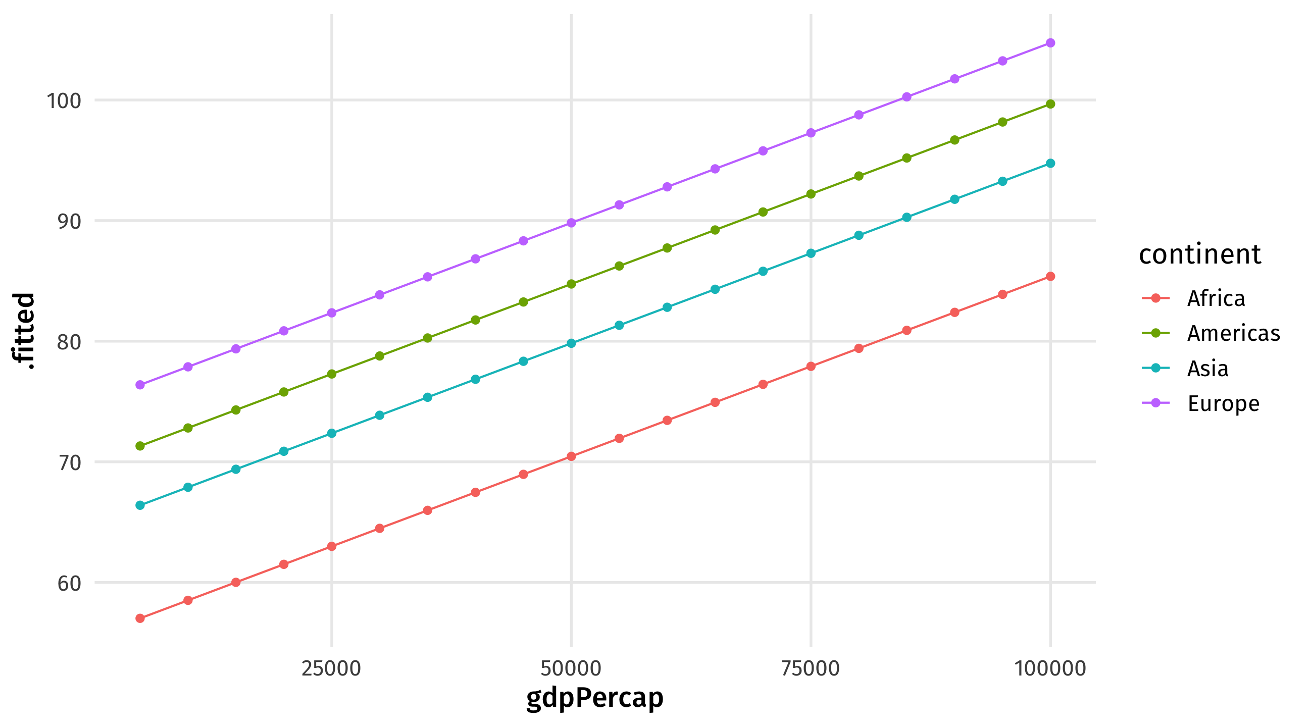
How different would this all look in different continents? We can vary continents too:

life_continent_scenario = crossing(gdpPercap = seq(from = 5000, to = 100000, by = 5000), 
                       pop = 20000000, year = 2005, 
                       continent = c("Asia", "Africa", "Americas", "Europe")) 
augment(life_model, newdata = life_continent_scenario)

# A tibble: 80 × 5
   gdpPercap      pop  year continent .fitted
       <dbl>    <dbl> <dbl> <chr>       <dbl>
 1      5000 20000000  2005 Africa       57.0
 2      5000 20000000  2005 Americas     71.3
 3      5000 20000000  2005 Asia         66.4
 4      5000 20000000  2005 Europe       76.4
 5     10000 20000000  2005 Africa       58.5
 6     10000 20000000  2005 Americas     72.8
 7     10000 20000000  2005 Asia         67.9
 8     10000 20000000  2005 Europe       77.9
 9     15000 20000000  2005 Africa       60.0
10     15000 20000000  2005 Americas     74.3
# ℹ 70 more rows

Predicting health

We can then save our predictions as an object, and plot them:

pred_health = augment(life_model, newdata = life_continent_scenario)
ggplot(pred_health, aes(x = gdpPercap, y = .fitted, color = continent)) + 
  geom_point() + geom_line()

Your turn: 🧑‍🎨 Art 🧑‍🎨

Let’s look at art from {juanr}: a dataset of auction sales records, including artists’ attributes, and market information

Sample from {art}.
artist_name	lot_title	event_year	nationality	real_price_usd
Ai Weiwei	Map of China	2006	Chinese	162293
Ai Weiwei	Coloured pots	2006	Chinese	106772
Ai Weiwei	Untitled	2006	Chinese	51250
Ai Weiwei	Gift from Beijing	2006	Chinese	8115
Ai Weiwei	Crossed tables	2007	Chinese	63041
Ai Weiwei	Chandelier	2007	Chinese	456791

Your turn: 🧑‍🎨 Art 🧑‍🎨

Using art:

Fit a model that predicts the sale price of the artwork (real_price_usd) using the year the artwork was created, the genre, the size, whether the artist is male or female, and whether the artist whent to an elite art school.
How much should we expect a painting to sell for if it was created in 2000, is a sculpture, is 360 inches, painted by a male artist who went to an elite art school?
Hold everything else constant and vary the art piece size from the smallest to the largest in the dataset. Visualize the price change.

10:00

How right are we?

Prediction accuracy

The question with prediction is always: how accurate were we?
If our model is predicting the outcome accurately that might be:
- a good sign that we are modeling the process that generates the outcome well
- useful for forcasting the future, or situations we don’t know about

Comparing to reality

How good are our model’s predictions?

We could compare our estimate of life expectancy to a real country, say Jamaica in 2007:

country	continent	year	lifeExp	pop	gdpPercap
Jamaica	Americas	2007	72.567	2780132	7320.88

We can use Jamaica’s values as our scenario, and see what our model predicted:

jamaica = crossing(continent = "Americas", year = 2007, pop = 2780132, gdpPercap = 7321)

Pretty close

Actual:

country	continent	year	lifeExp	pop	gdpPercap
Jamaica	Americas	2007	72.567	2780132	7320.88

Estimate:

augment(life_model, newdata = jamaica)

# A tibble: 1 × 5
  continent  year     pop gdpPercap .fitted
  <chr>     <dbl>   <dbl>     <dbl>   <dbl>
1 Americas   2007 2780132      7321    72.5

Is this really a prediction?

Our estimate of Jamaica is not really prediction, since we used that observation to fit our model
This is an in-sample prediction $\rightarrow$ seeing how well our model does at predicting the data that we used to generate it
“True” prediction is out-of-sample $\rightarrow$ using a model to generate predictions about something that hasn’t happened yet

Figure. Is catch and release really fishing?

Out of sample prediction

Imagine in the year 1957 we fit a model with the info we had available at the time:

gap_57 = gapminder %>% filter(year <= 1957)
mod_57 = lm(lifeExp ~ gdpPercap + pop + continent + year, data = gap_57)

Now it’s 2007, someone finds the model, and wants to know: how well could this model have predicted the future?

jamaica = crossing(continent = "Americas", year = 2007, pop = 2780132, gdpPercap = 7321)

This is an out-of-sample prediction: our model has data before 1957, but our prediction is based off of Jamaica’s characteristics in 2007

How did we do?

Jamaica in 2007:

country	continent	year	lifeExp	pop	gdpPercap
Jamaica	Americas	2007	72.6	2780132	7320.9

What our first model with all the data predicted, 2007 included (in sample):

continent	year	pop	gdpPercap	.fitted
Americas	2007	2780132	7321	72.5

What our 1957 model predicted for 2007 (out of sample):

continent	year	pop	gdpPercap	.fitted
Americas	2007	2780132	7321	79.8

Out of sample prediction is generally worse

As a general rule, models will tend to perform worse out-of-sample than in-sample

This is because the model is over-fitting the data $\rightarrow$ tailoring the model equation too closely to the data we have

Something could change that our data doesn’t know about, or…

Our model could over-emphasize patterns that don’t generalize to new data

You can’t time the market

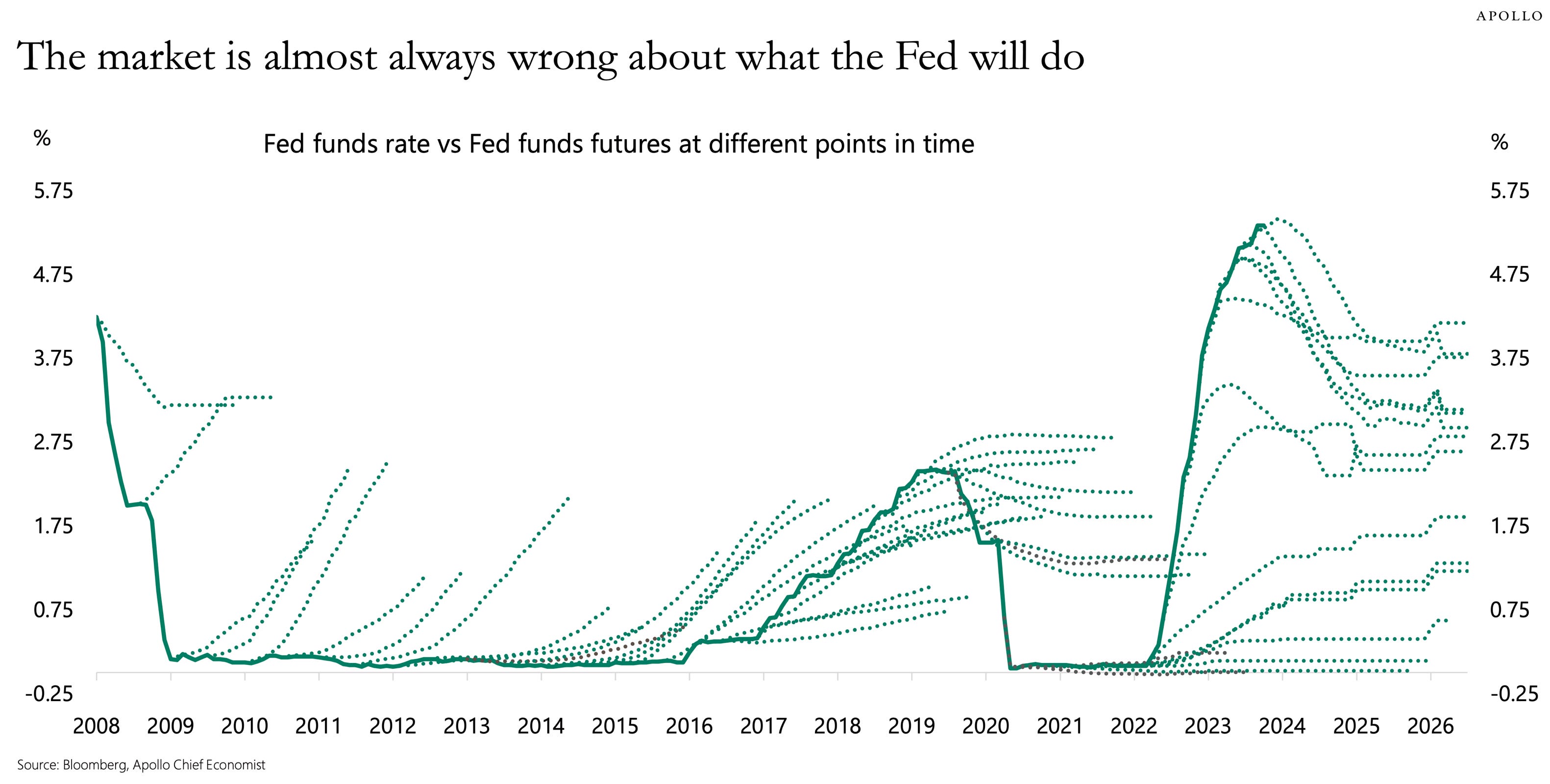
Lesson: buy index funds, set it and forget it

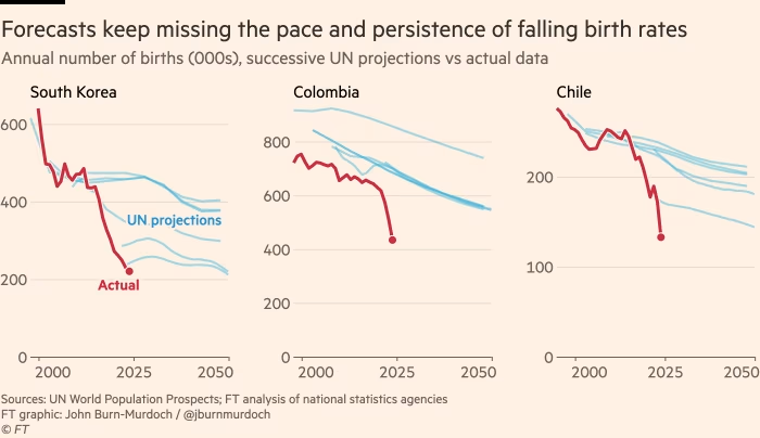
Why are we so wrong about fertility?

🚨 Your turn: 🎥 The movies 🎥🚨

Using movies:

Fit a model that predicts gross (outcome) using genre1, duration, budget, year, imdb_score, and whether or not it’s in color.
Look up a movie in the dataset. How well does the model predict a movie that shares that movie’s characteristics?
Look up a movie on IMDB that came out after the data ends (2016). How well does your model predict that movie’s gross?

10:00