Data wrangling II

POL51

Juan Tellez

jftellez@ucdavis.edu

UC Davis

October 9, 2024

Get ready

Boot up Posit Cloud
Download the script for today’s examples
- Schedule ➡️ Example ➡️ Today
Upload the script to Posit Cloud

Plan for today

Making amends + objects review

Mutating new variables

Creating categories

Weekly check-in

So far, you:

somehow do not know how to make every graph from scratch based solely off memory

are confused about errors you are seeing for the first time in a computer program you’ve never used before

are unable to re-type all the code I am presenting on slides into your notes at what would be a rate on par with a professional court stenographer

Weekly check-in

You are confused and unsure of yourselves

But you are doing well

You’ve only been coding for two weeks

You just need to know how to piece together answers from notes + slides

You will slowly get better at coding, and dealing with errors (be patient!)

Back to objects

Using objects

ggplot(gapminder, aes(x = gdpPercap, y = lifeExp)) + geom_point()

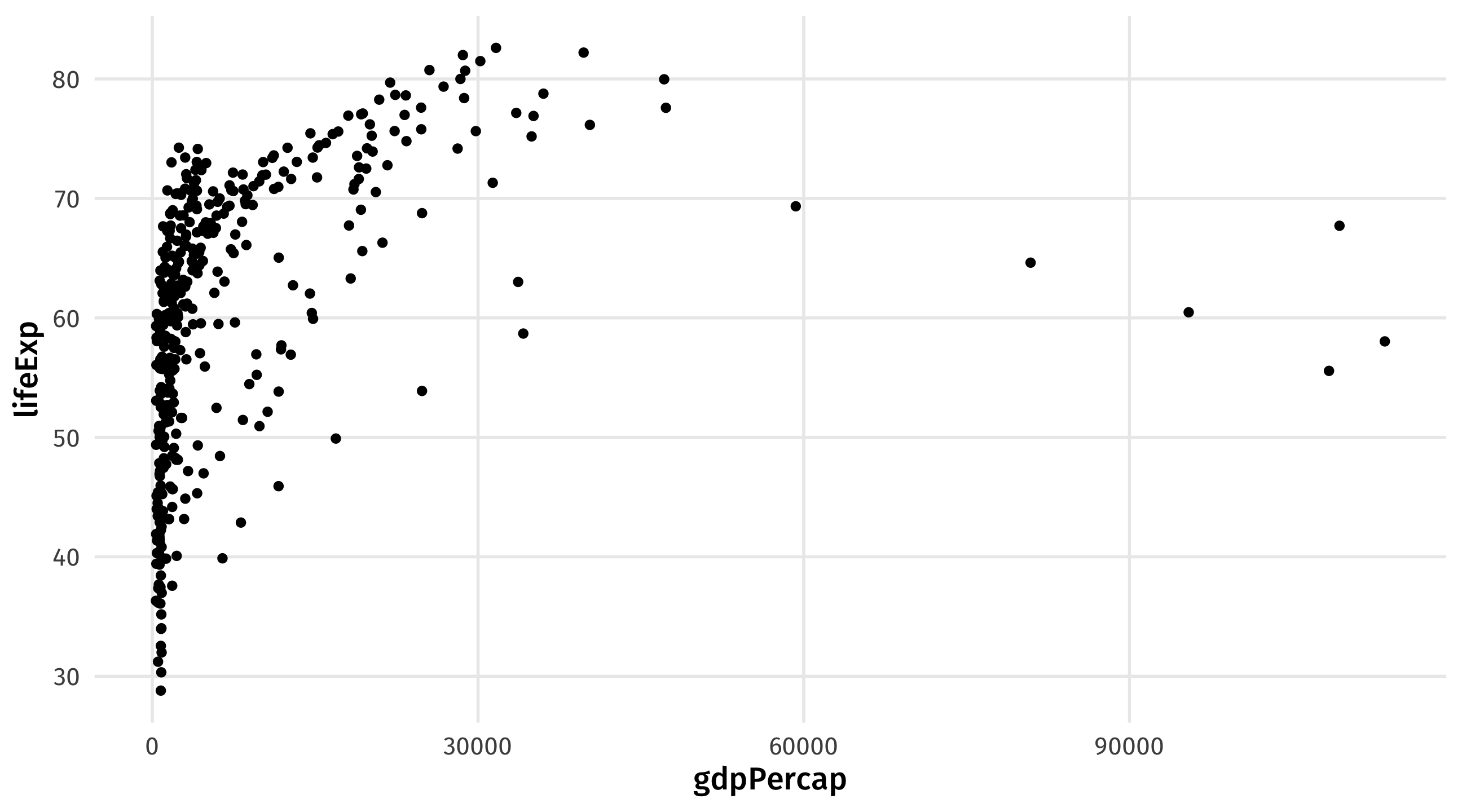
What if I wanted to make this same plot, but only looking at countries in Asia?

Subset to Asia

I can use filter() to subset the data to Asia, store it as a new object gap_asia, and use that new object to make a plot

gap_asia = gapminder |>
    filter(continent == "Asia")

ggplot(gap_asia, aes(x = gdpPercap, y = lifeExp)) + geom_point()

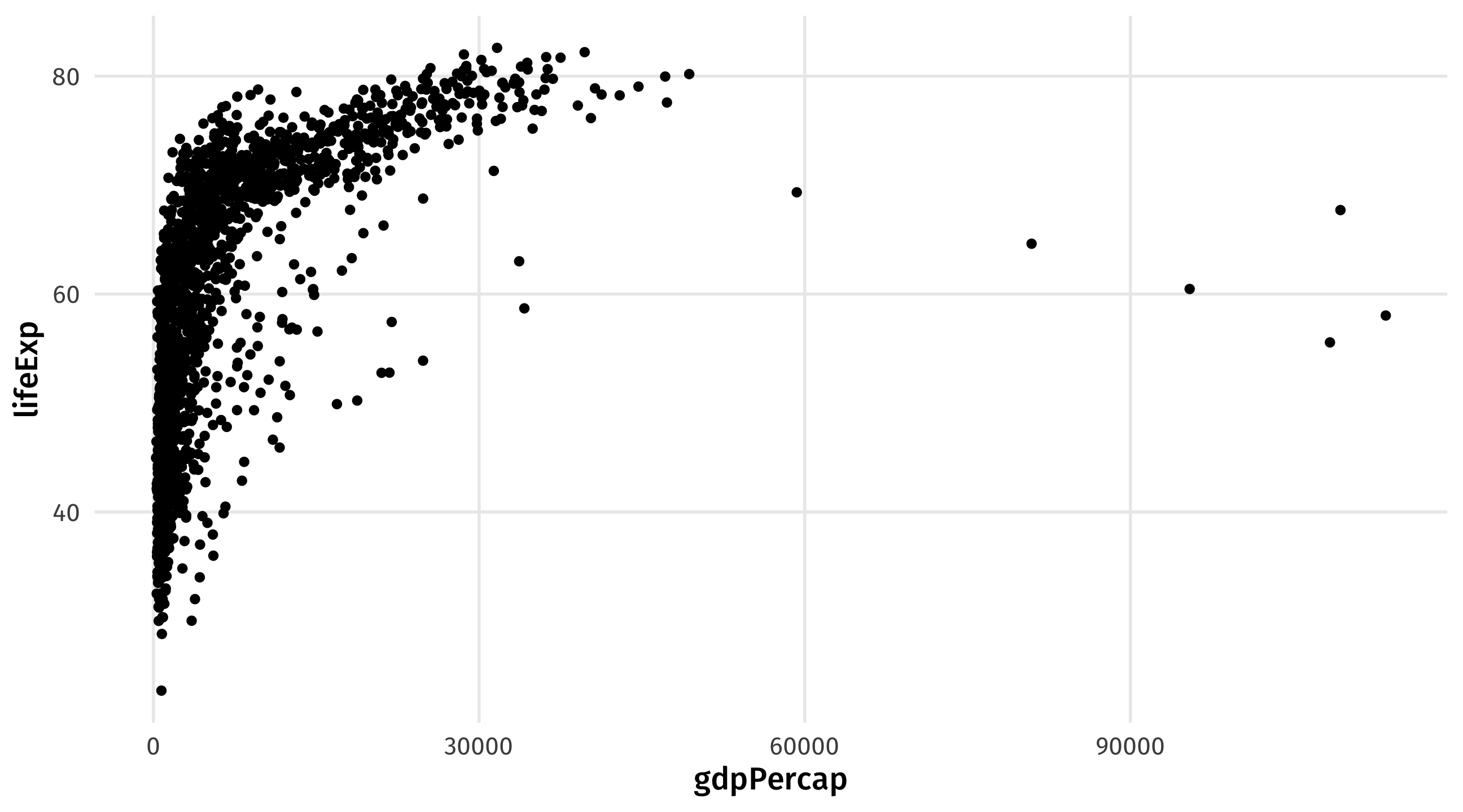
Using the new object

Notice how I need to use the new object

the original gapminder does not have what I want

ggplot(gap_asia, aes(x = gdpPercap, y = lifeExp)) + geom_point()

ggplot(gapminder, aes(x = gdpPercap, y = lifeExp)) + geom_point()

filter() and variables types

Filtering requires knowing the type of variable you are working with

Numerical variables do not use quotes

gapminder |>
    filter(year > 2000)

Categorical variables use quotes, and spelling must be exact

✅

gapminder |>
    filter(continent == "Asia")

❌

gapminder |>
    filter(continent == "asia")

Logical variables

TRUE/FALSE variables are all-caps, no quotes

apples |>
    filter(sweet == TRUE)

Mutating variables

Homicides in 2019

state	city	population	murder_total
Alabama	Mobile	248431	50
Alaska	Anchorage	296188	27
Arizona	Chandler	249355	5
Arizona	Gilbert	242090	5
Arizona	Glendale	249273	12
Arizona	Mesa	492268	23

Most violent cities in America?

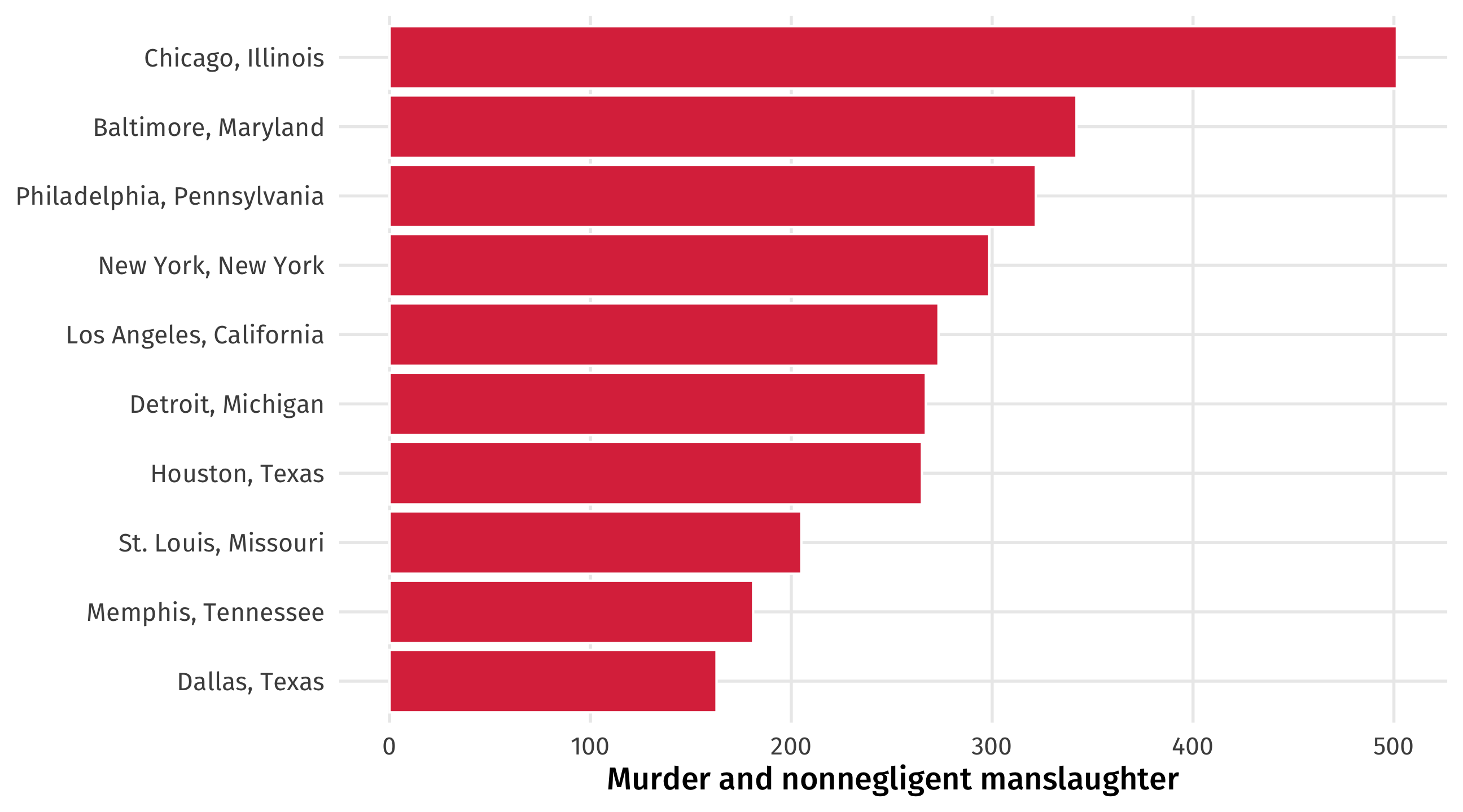
Fewer deaths in towns with less people

Normalizing variables

To compare across cities we need to take into account differences in population

We want to know how many murders have taken place (or drug overdoses, or crimes, or COVID cases, or…) per person in the city (per capita)

This is called normalizing a variable; changing it so that we can make units more comparable

Murder rate

In math terms this is just dividing the number of murders by population:

\(Murders_{capita} = \frac{Murders}{Population}\) = “how many murders per person”

Since this fraction is tiny, the convention is to multiply by a number that makes sense

for the population of a city, say 100,000 people

\(Murders_{per 100k} = \frac{Murders}{Population} \times 100,000\) = “how many murders per 100,000 people”

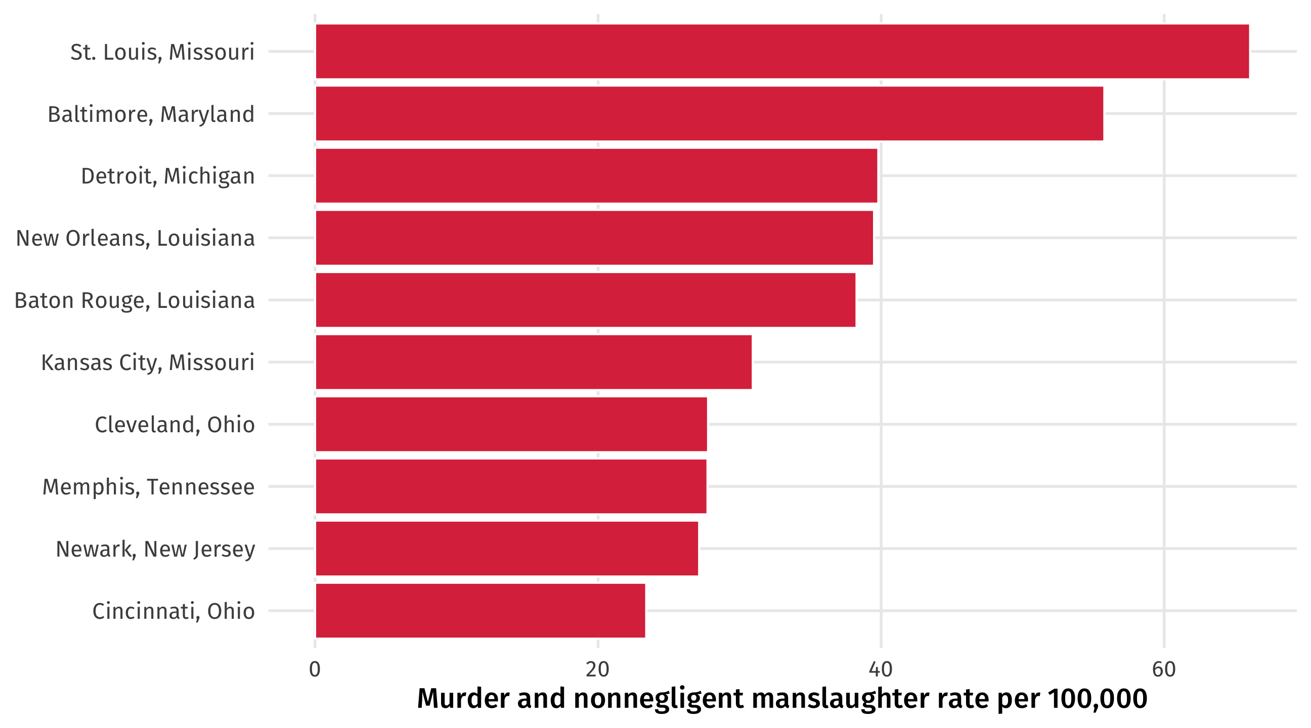
Comparing murder rates

If we look at murder rates, the picture changes:

Making new variables with `mutate()`

mutate() adds new variables to data

Using mutate

murder_set

# A tibble: 100 × 4
   state      city       population murder_total
   <chr>      <chr>           <dbl>        <dbl>
 1 Alabama    Mobile         248431        50.0 
 2 Alaska     Anchorage      296188        27.0 
 3 Arizona    Chandler       249355         5.01
 4 Arizona    Gilbert        242090         5.01
 5 Arizona    Glendale       249273        12.0 
 6 Arizona    Mesa           492268        23.0 
 7 Arizona    Phoenix       1608139       154.  
 8 Arizona    Scottsdale     251840         5.01
 9 Arizona    Tucson         532323        46.0 
10 California Anaheim        353400        10.0 
# ℹ 90 more rows

Note

murder_set is the name of the homicide data

Using mutate

murder_set |>
    mutate()

# A tibble: 100 × 4
   state      city       population murder_total
   <chr>      <chr>           <dbl>        <dbl>
 1 Alabama    Mobile         248431        50.0 
 2 Alaska     Anchorage      296188        27.0 
 3 Arizona    Chandler       249355         5.01
 4 Arizona    Gilbert        242090         5.01
 5 Arizona    Glendale       249273        12.0 
 6 Arizona    Mesa           492268        23.0 
 7 Arizona    Phoenix       1608139       154.  
 8 Arizona    Scottsdale     251840         5.01
 9 Arizona    Tucson         532323        46.0 
10 California Anaheim        353400        10.0 
# ℹ 90 more rows

Using mutate

murder_set |>
    mutate(murder_capita = murder_total/population)

# A tibble: 100 × 5
   state      city       population murder_total murder_capita
   <chr>      <chr>           <dbl>        <dbl>         <dbl>
 1 Alabama    Mobile         248431        50.0      0.000201 
 2 Alaska     Anchorage      296188        27.0      0.0000912
 3 Arizona    Chandler       249355         5.01     0.0000201
 4 Arizona    Gilbert        242090         5.01     0.0000207
 5 Arizona    Glendale       249273        12.0      0.0000481
 6 Arizona    Mesa           492268        23.0      0.0000467
 7 Arizona    Phoenix       1608139       154.       0.0000955
 8 Arizona    Scottsdale     251840         5.01     0.0000199
 9 Arizona    Tucson         532323        46.0      0.0000864
10 California Anaheim        353400        10.0      0.0000283
# ℹ 90 more rows

Notice that I named a new variable, murder_capita

Using mutate

murder_set |>
    mutate(murder_capita = murder_total/population, murder_rate = murder_capita *
        1e+05)

# A tibble: 100 × 6
   state      city       population murder_total murder_capita murder_rate
   <chr>      <chr>           <dbl>        <dbl>         <dbl>       <dbl>
 1 Alabama    Mobile         248431        50.0      0.000201        20.1 
 2 Alaska     Anchorage      296188        27.0      0.0000912        9.12
 3 Arizona    Chandler       249355         5.01     0.0000201        2.01
 4 Arizona    Gilbert        242090         5.01     0.0000207        2.07
 5 Arizona    Glendale       249273        12.0      0.0000481        4.81
 6 Arizona    Mesa           492268        23.0      0.0000467        4.67
 7 Arizona    Phoenix       1608139       154.       0.0000955        9.55
 8 Arizona    Scottsdale     251840         5.01     0.0000199        1.99
 9 Arizona    Tucson         532323        46.0      0.0000864        8.64
10 California Anaheim        353400        10.0      0.0000283        2.83
# ℹ 90 more rows

Notice the new columns

Forgetting to store

If you don’t store your changes, they will melt away, like tears in the rain

murder_set |>
    mutate(murder_capita = murder_total/population, murder_rate = murder_capita *
        1e+05)

murder_set

# A tibble: 100 × 4
   state      city       population murder_total
   <chr>      <chr>           <dbl>        <dbl>
 1 Alabama    Mobile         248431        50.0 
 2 Alaska     Anchorage      296188        27.0 
 3 Arizona    Chandler       249355         5.01
 4 Arizona    Gilbert        242090         5.01
 5 Arizona    Glendale       249273        12.0 
 6 Arizona    Mesa           492268        23.0 
 7 Arizona    Phoenix       1608139       154.  
 8 Arizona    Scottsdale     251840         5.01
 9 Arizona    Tucson         532323        46.0 
10 California Anaheim        353400        10.0 
# ℹ 90 more rows

New object, or overwite the old one?

When you mutate(), you should overwrite the original data by naming the “new” object the same as the “old” one

murder_set = murder_set |>
    mutate(murder_capita = murder_total/population, murder_rate = murder_capita *
        1e+05)

This way, you add columns to your original dataset

murder_set

# A tibble: 100 × 6
   state      city       population murder_total murder_capita murder_rate
   <chr>      <chr>           <dbl>        <dbl>         <dbl>       <dbl>
 1 Alabama    Mobile         248431        50.0      0.000201        20.1 
 2 Alaska     Anchorage      296188        27.0      0.0000912        9.12
 3 Arizona    Chandler       249355         5.01     0.0000201        2.01
 4 Arizona    Gilbert        242090         5.01     0.0000207        2.07
 5 Arizona    Glendale       249273        12.0      0.0000481        4.81
 6 Arizona    Mesa           492268        23.0      0.0000467        4.67
 7 Arizona    Phoenix       1608139       154.       0.0000955        9.55
 8 Arizona    Scottsdale     251840         5.01     0.0000199        1.99
 9 Arizona    Tucson         532323        46.0      0.0000864        8.64
10 California Anaheim        353400        10.0      0.0000283        2.83
# ℹ 90 more rows

New object, or overwite the old one?

When we filter(), we want to create a new object

If we overwrite the original object, we lose the original data

❌

gapminder = gapminder |>
    filter(continent == "Africa")
gapminder

# A tibble: 624 × 6
   country continent  year lifeExp      pop gdpPercap
   <fct>   <fct>     <int>   <dbl>    <int>     <dbl>
 1 Algeria Africa     1952    43.1  9279525     2449.
 2 Algeria Africa     1957    45.7 10270856     3014.
 3 Algeria Africa     1962    48.3 11000948     2551.
 4 Algeria Africa     1967    51.4 12760499     3247.
 5 Algeria Africa     1972    54.5 14760787     4183.
 6 Algeria Africa     1977    58.0 17152804     4910.
 7 Algeria Africa     1982    61.4 20033753     5745.
 8 Algeria Africa     1987    65.8 23254956     5681.
 9 Algeria Africa     1992    67.7 26298373     5023.
10 Algeria Africa     1997    69.2 29072015     4797.
# ℹ 614 more rows

New object, or overwite the old one?

Make a new object instead:

✅

gap_africa = gapminder |>
    filter(continent == "Africa")
gap_africa

# A tibble: 624 × 6
   country continent  year lifeExp      pop gdpPercap
   <fct>   <fct>     <int>   <dbl>    <int>     <dbl>
 1 Algeria Africa     1952    43.1  9279525     2449.
 2 Algeria Africa     1957    45.7 10270856     3014.
 3 Algeria Africa     1962    48.3 11000948     2551.
 4 Algeria Africa     1967    51.4 12760499     3247.
 5 Algeria Africa     1972    54.5 14760787     4183.
 6 Algeria Africa     1977    58.0 17152804     4910.
 7 Algeria Africa     1982    61.4 20033753     5745.
 8 Algeria Africa     1987    65.8 23254956     5681.
 9 Algeria Africa     1992    67.7 26298373     5023.
10 Algeria Africa     1997    69.2 29072015     4797.
# ℹ 614 more rows

🚨 Your turn 🌡️ Climate change 🌡️ 🚨

Sample from climate dataset
country	year	population	co2
Kyrgyzstan	1863	784425	0.00
Ireland	1879	5186259	NA
Ghana	1993	16106756	4.31
Reunion	1975	484785	0.48
Taiwan	1995	21356026	168.87

🚨 Your turn 🌡️ Climate change 🌡️ 🚨

Using climate, make the following two plots looking only at the United States and China:

A grouped time-series of co2 emissions over time (separate country by color)
A grouped time-series of co2 emissions per capita over time (separate country by color)
Who’s to “blame” for climate change? And where should we focus environmental efforts?

10:00

Creating categories

Sometimes we want to create categorical variables out of continuous ones

Why? Categories are sometimes clearer: this city is “high crime”, this city is “low crime”

Sometimes all that matters is some outcome: who won the election?

Who won the county?

sample from elections dataset
name	state	per_gop_2020	per_dem_2020
Polk County	AR	0.83	0.15
Grant County	NE	0.93	0.05
Columbia County	FL	0.72	0.27
Graves County	KY	0.78	0.21
San Bernardino County	CA	0.44	0.54
McKean County	PA	0.72	0.26
Gibson County	TN	0.73	0.26
Hudspeth County	TX	0.67	0.32
Erie County	OH	0.55	0.43
Washington County	KS	0.82	0.16

Creating categories

We can use case_when() in conjunction with mutate() to create categorical variables

Like filter(), case_when() also relies on logical operators

start by making new variable with mutate()

small_elections |>
    mutate()

# A tibble: 3,152 × 4
   name            state per_gop_2020 per_dem_2020
   <chr>           <chr>        <dbl>        <dbl>
 1 Autauga County  AL           0.714       0.270 
 2 Baldwin County  AL           0.762       0.224 
 3 Barbour County  AL           0.535       0.458 
 4 Bibb County     AL           0.784       0.207 
 5 Blount County   AL           0.896       0.0957
 6 Bullock County  AL           0.248       0.747 
 7 Butler County   AL           0.575       0.418 
 8 Calhoun County  AL           0.688       0.298 
 9 Chambers County AL           0.573       0.416 
10 Cherokee County AL           0.860       0.132 
# ℹ 3,142 more rows

Who won the county?

The general formula: case_when(CONDITION ~ LABEL)

small_elections |>
    mutate(who_won = case_when(per_gop_2020 > per_dem_2020 ~ "Republicans"))

# A tibble: 3,152 × 5
   name            state per_gop_2020 per_dem_2020 who_won    
   <chr>           <chr>        <dbl>        <dbl> <chr>      
 1 Autauga County  AL           0.714       0.270  Republicans
 2 Baldwin County  AL           0.762       0.224  Republicans
 3 Barbour County  AL           0.535       0.458  Republicans
 4 Bibb County     AL           0.784       0.207  Republicans
 5 Blount County   AL           0.896       0.0957 Republicans
 6 Bullock County  AL           0.248       0.747  <NA>       
 7 Butler County   AL           0.575       0.418  Republicans
 8 Calhoun County  AL           0.688       0.298  Republicans
 9 Chambers County AL           0.573       0.416  Republicans
10 Cherokee County AL           0.860       0.132  Republicans
# ℹ 3,142 more rows

““Republicans” will be assigned to the who_won variable if per_gop_2020 is greater than per_dem_2020”

Who won the county?

The general formula: case_when(CONDITION ~ LABEL)

small_elections |>
    mutate(who_won = case_when(per_gop_2020 > per_dem_2020 ~ "Republicans", per_dem_2020 >
        per_gop_2020 ~ "Democrats"))

# A tibble: 3,152 × 5
   name            state per_gop_2020 per_dem_2020 who_won    
   <chr>           <chr>        <dbl>        <dbl> <chr>      
 1 Autauga County  AL           0.714       0.270  Republicans
 2 Baldwin County  AL           0.762       0.224  Republicans
 3 Barbour County  AL           0.535       0.458  Republicans
 4 Bibb County     AL           0.784       0.207  Republicans
 5 Blount County   AL           0.896       0.0957 Republicans
 6 Bullock County  AL           0.248       0.747  Democrats  
 7 Butler County   AL           0.575       0.418  Republicans
 8 Calhoun County  AL           0.688       0.298  Republicans
 9 Chambers County AL           0.573       0.416  Republicans
10 Cherokee County AL           0.860       0.132  Republicans
# ℹ 3,142 more rows

““Republicans” will be assigned to the who_won variable if per_gop_2020 is greater than per_dem_2020. “Democrats” will be assigned if per_dem_2020 is greater than per_gop_2020“.

Tradeoff: clarity vs. complexity

Turning continuous variables into categories can make the “big picture” clearer

How many counties did each party win?

Who won the county?
who_won	n	percentage
Democrats	557	17.67132
Republicans	2595	82.32868

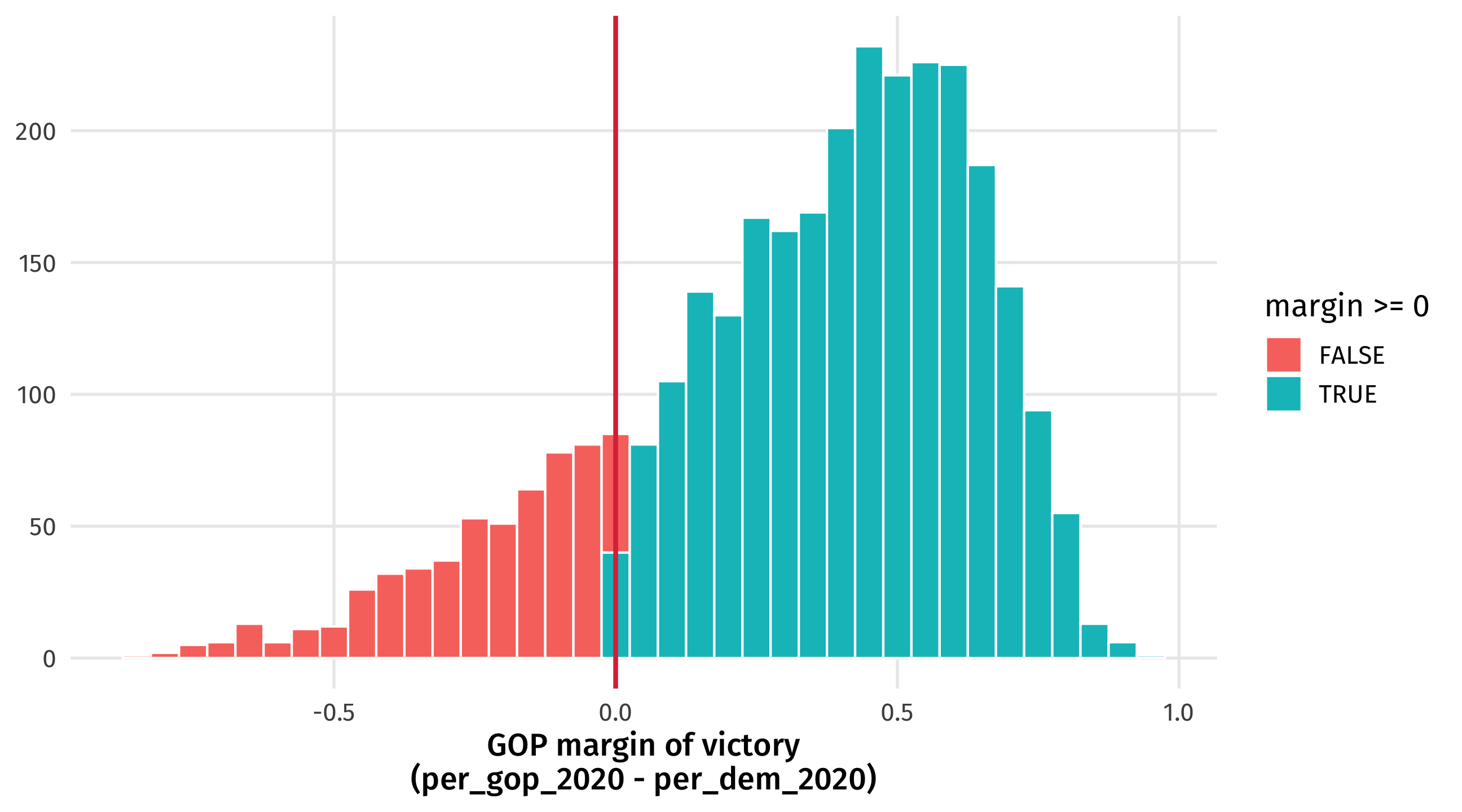
Tradeoff: clarity vs. complexity

But we lose complexity: how much did each party win by?

🚨 Your turn 🚨

Using the elections dataset:

Create a variable that tells you what happened in the 2016 election in each county. The variable should incorporate four possibilities:
1. DEMS won in 2012 and in 2016 (“true blue”)
2. REPS won in 2012 and in 2016 (“true red”)
3. the county flipped from blue to red (“blue to red”)
4. the county flipped from red to blue (“red to blue”)

15:00

Data wrangling II

Get ready

Plan for today

Weekly check-in

Weekly check-in

Back to objects

Using objects

Subset to Asia

Using the new object

filter() and variables types

Logical variables

Mutating variables

Homicides in 2019

Most violent cities in America?

Fewer deaths in towns with less people

Normalizing variables

Murder rate

Comparing murder rates

Making new variables with mutate()

Using mutate

Using mutate

Using mutate

Using mutate

Forgetting to store

New object, or overwite the old one?

New object, or overwite the old one?

New object, or overwite the old one?

🚨 Your turn 🌡️ Climate change 🌡️ 🚨

🚨 Your turn 🌡️ Climate change 🌡️ 🚨

Creating categories

Creating categories

Who won the county?

Creating categories

Who won the county?

Who won the county?

Tradeoff: clarity vs. complexity

Tradeoff: clarity vs. complexity

🚨 Your turn 🚨

Making new variables with `mutate()`