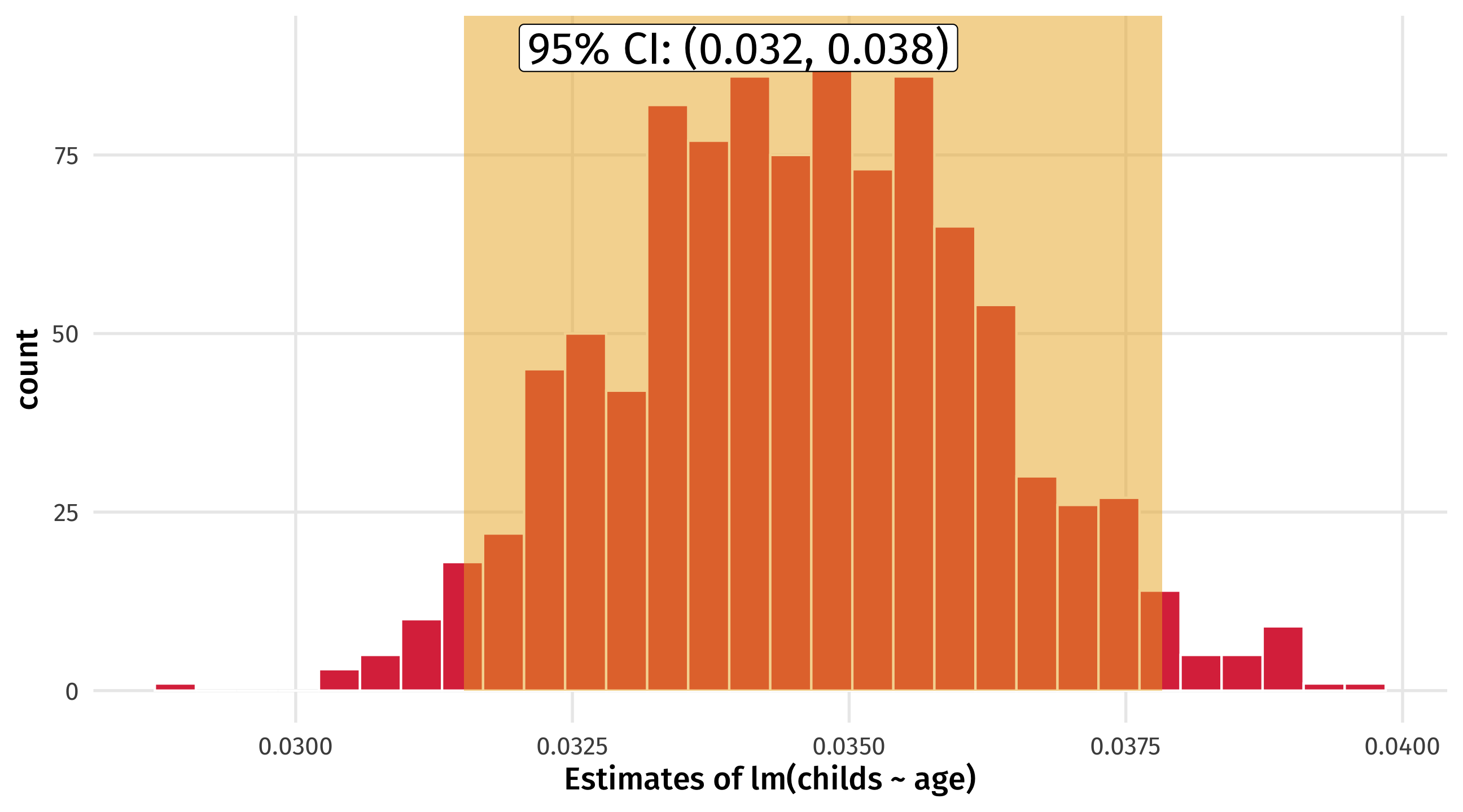
We can also look at the 95% confidence interval – we are 95% “confident” the effect of age on the number of children a person has is between .032 and .038
Uncertainty in R
lm() will estimate the standard error of regression estimates for us using the statistical theory approach, but the results are similar to boostrapping
mod =lm(obama ~ sex, data = gss_sm)tidy(mod)
term
estimate
std.error
statistic
p.value
(Intercept)
0.576
0.0177
32.6
5.84e-182
sexFemale
0.0871
0.0234
3.72
0.000206
Uncertainty in R
We can also ask tidy for the 95% CI:
tidy(mod, conf.int =TRUE)
term
estimate
std.error
statistic
p.value
conf.low
conf.high
(Intercept)
0.576
0.0177
32.6
5.84e-182
0.541
0.611
sexFemale
0.0871
0.0234
3.72
0.000206
0.0412
0.133
conf.low and conf.high are the lower and upper bound of the 95% CI
Statistical significance
The last (and most controversial) way to quantify uncertainty is statistical significance
We want to make a binary decision: are we confident enough in this estimate to say that it is significant?
Or are we too uncertain, given sampling variability?
Is the result significant, or not significant?
Can you persuade voters?
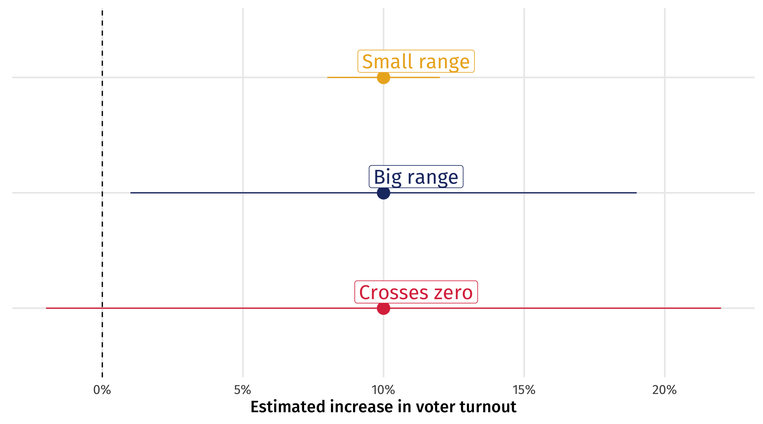
Imagine we run an experiment on TV ads, estimate the effect of the treatment on voter turnout, and the 95% confidence interval for that effect
The experiment went well so we are confident in causal sense, but there is still uncertainty from sampling
Three scenarios
Three scenarios for the results: same effect size, different 95% CIs
How much should we worry?
Small range: great! Effect is precise; ads are worth it!
Big range: OK-ish! Effect could be tiny, or huge; are the ads worth it? At least we know they help (positive)
Crosses zero: awful! Ads could work (+), they could do nothing (0), or they could be counterproductive (-)
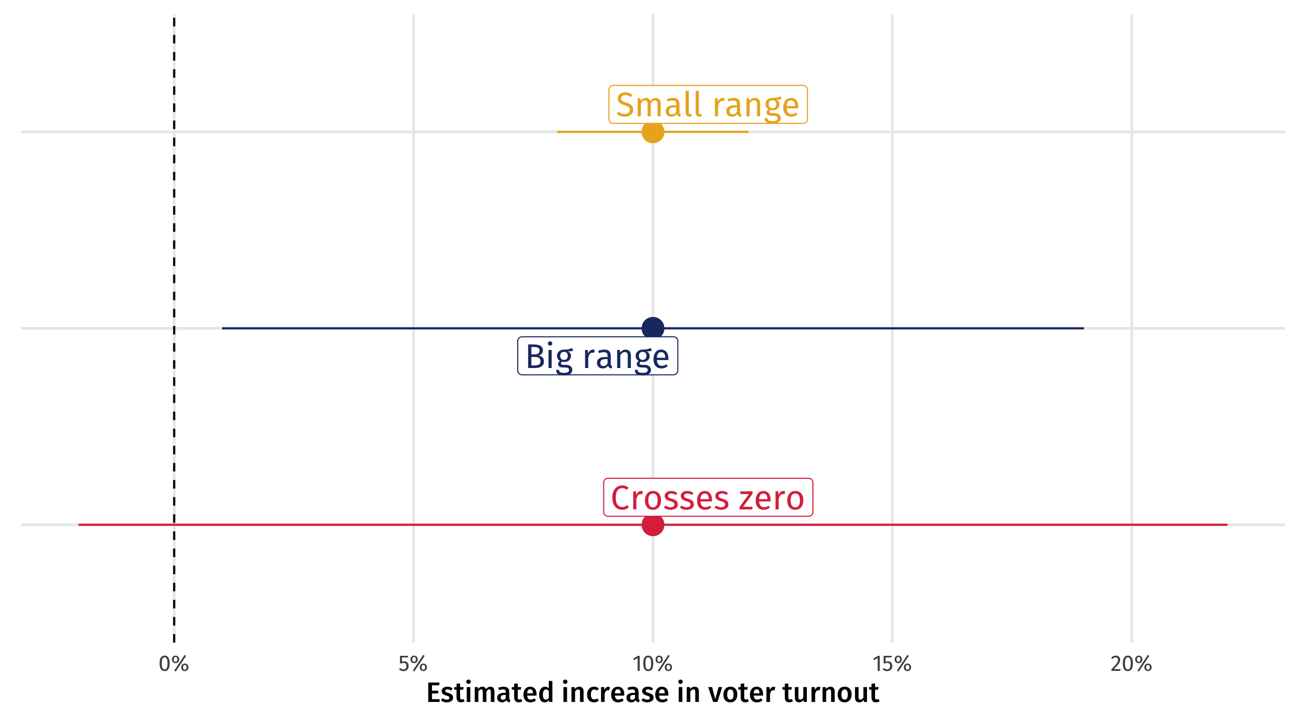
Crossing zero: the worst scenario
When the 95% CI crosses zero we are so uncertain we are unsure whether effect is positive, zero, or negative
Researchers worry so much about this that it is conventional to report whether the 95% CI of an effect estimate crosses zero
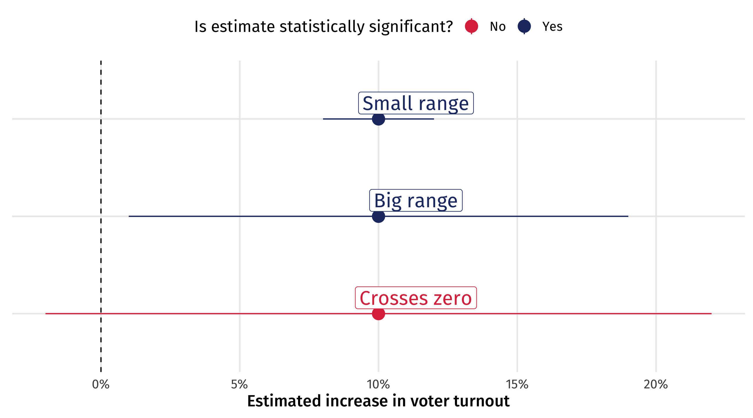
When a 95% CI for an estimate doesn’t cross zero, we say that the estimate is statistically significant
If the 95% CI crosses zero, the estimate is not statistically significant
Statistical significance
Hypothesis testing
Statistical significance is at the center of hypothesis testing
Researcher wants to decide between two possibilities:
null hypothesis (\(H_0\)): the ad has no effect on turnout
alternative hypothesis (\(H_a\)): the ad has some effect on turnout
A statistically significant estimate rejects the null
Remember this is all about sampling uncertainty, not causality!
Arbitrary?
You could have an estimate with a 95% CI that barely escapes crossing zero, and call that statistically significant
And another estimate with a 95% CI that barely crosses zero, and call that not statistically significant
That’s pretty arbitrary!
And it all hinges on the size of the confidence interval
if we made a 98% CI, or a 95.1% CI, we might conclude different things are and aren’t significant
The 95% CI is a convention; where does it come from?
The arbitrary nature of “significance testing”
Fisher (1925), who came up with it, says:
It is convenient to take this point [95% CI] as a limit in judging whether [an effect] is to be considered significant or not. (Fisher 1925)
But that other options are plausible:
If one in twenty [95% CI] does not seem high enough odds, we may, if we prefer it, draw the line at one in fifty [98% CI]… or one in a hundred [99% CI]…Personally, the writer prefers…[95% CI] (Fisher 1926)
The significance testing controversy
So arbitrary; why make this binary distinction?
Sometimes we have to make the call:
when is a baby’s temperature so high that you should give them medicine?
100.4 is a useful (arbitrary) threshold for action
This is a huge topic of debate in social science, other proposals we can’t cover:
redefining how we think about probability
focusing on estimate sizes
focusing on likely range of estimates
Statistical significance in R
The stars (*) in regression output tell you whether an estimate’s confidence interval crosses zero and at what level of confidence
This is done with the p-value (which we don’t cover), the mirror image of the confidence interval
Number of kids
(Intercept)
0.153
(0.086)
age
0.035 ***
(0.002)
nobs
2849
*** p < 0.001; ** p < 0.01; * p < 0.05.
Reading the stars
(*) p < .05 = the 95% confidence interval does not cross zero
(**) p < .01 = the 99% confidence interval does not cross zero
(***) p < .001 = the 99.9% confidence interval does not cross zero
Number of kids
(Intercept)
0.153
(0.086)
age
0.035 ***
(0.002)
nobs
2849
*** p < 0.001; ** p < 0.01; * p < 0.05.
Another way…
The estimate is statistically significant at the…
(*) p < .05 = the 95% confidence level
(**) p < .01 = the 99% confidence level
(***) p < .001 = the 99.9% confidence level
Number of kids
(Intercept)
0.153
(0.086)
age
0.035 ***
(0.002)
nobs
2849
*** p < 0.001; ** p < 0.01; * p < 0.05.
Making inferences with data
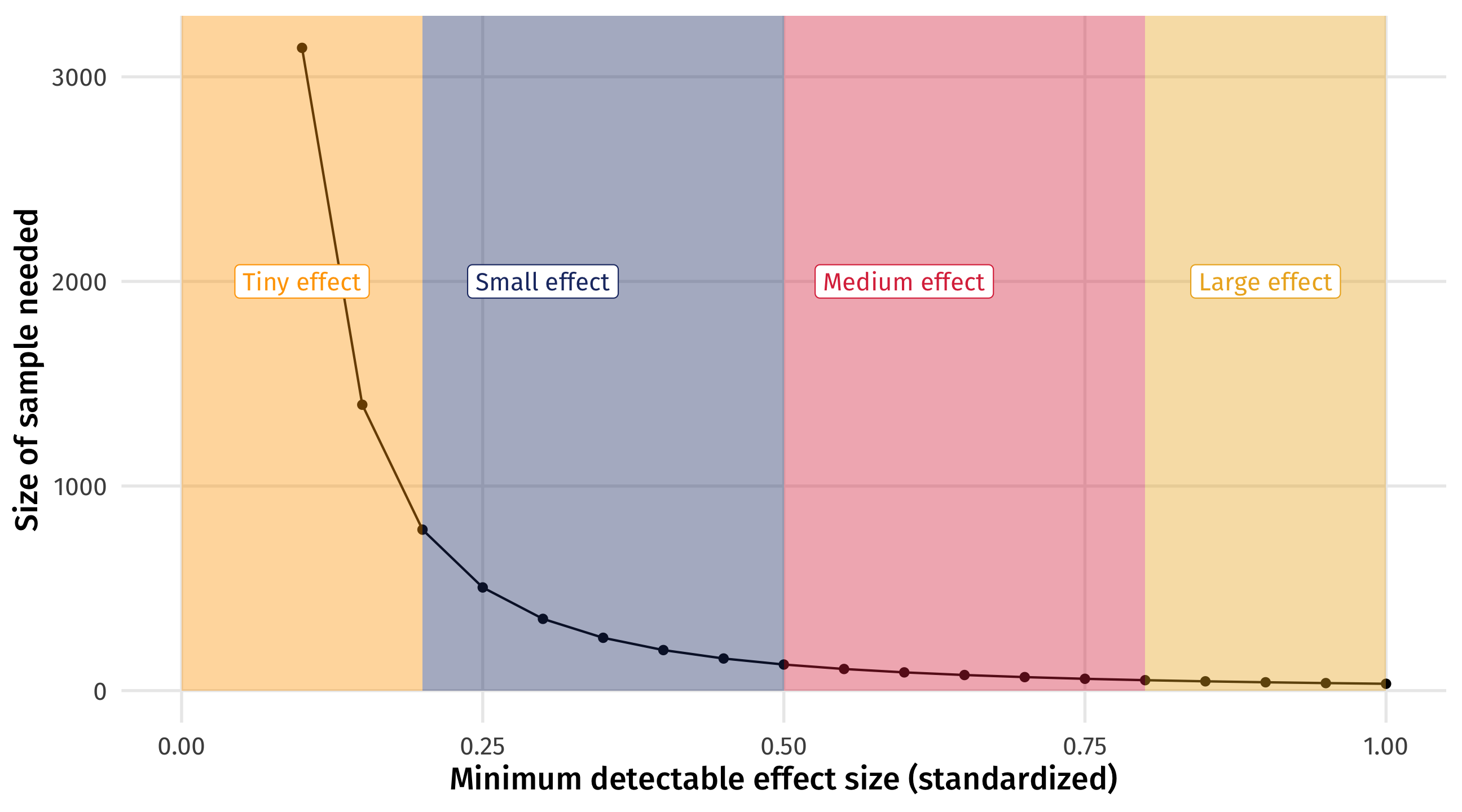
How much data do I need to estimate X?
With the Law of Large Numbers and simulation (or theory), we can figure out how much data we would need to reliably estimate an effect of a particular size
This is called power analysis
How much statistical power do we have, or need to answer our research question?
How much data do I need to estimate X?
You need less data to estimate larger effects
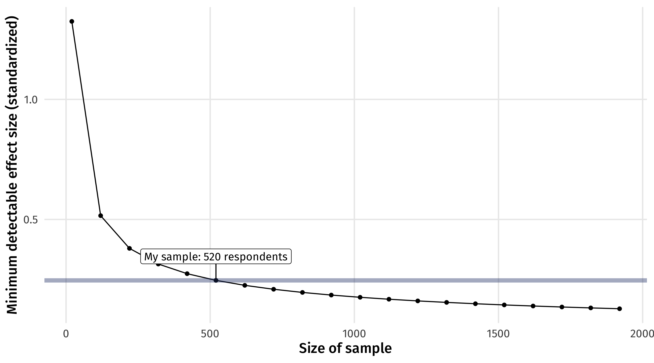
How good is my sample?
You can see how big (small) of an effect you can estimate given your data
Statistical significance and causalitly
When we control for a confounder, our treatment estimate can change a lot
In this case, shrinks closer to zero, but not perfectly; is there still “an effect”?
Naive model
Model with controls
(Intercept)
10708.3
-39456.6 ***
(6210.7)
(5223.1)
bathrooms
250326.5 ***
-5164.6
(2759.5)
(3519.5)
sqft_living
283.9 ***
(3.0)
nobs
21613
21613
*** p < 0.001; ** p < 0.01; * p < 0.05.
Statistical significance and causalitly
One (controversial) approach is to notice that the effect has shrunk closer to zero, so much so that it is no longer statistically significant
Naive model
Model with controls
(Intercept)
10708.3
-39456.6 ***
(6210.7)
(5223.1)
bathrooms
250326.5 ***
-5164.6
(2759.5)
(3519.5)
sqft_living
283.9 ***
(3.0)
nobs
21613
21613
*** p < 0.001; ** p < 0.01; * p < 0.05.
From the homework
In the naive model, the effect of children on affairs is positive and statistically significant
But once we control for the right confounds, the effect of children on affairs is negative and not statistically significant
This is one way (the correct) controls can help us make better inferences
Naive model
Controls model
(Intercept)
0.912 ***
0.562 *
(0.251)
(0.264)
childrenyes
0.760 *
-0.033
(0.297)
(0.358)
yearsmarried
0.112 ***
(0.029)
nobs
601
601
*** p < 0.001; ** p < 0.01; * p < 0.05.
Don’t forget
A lot of this hinges on that arbitrary 95% CI convention
Sometimes conventions are good and useful
But we shouldn’t forget they are conventions!
Pulling it all together
Where to go from here?
We’ve done a lot this quarter
Where to go from here?
Basics of data wrangling, visualization, and analysis
Modeling relationships between variables
Thinking and modeling causally
Making inferences with uncertainty
Keep learning R
Every Tuesday: free data + a visualization challenge + free code
Keep thinking causally
No randomization; who is being compared here?
But also: don’t be a lazy cynic! What is the confound?