| Sample | Avg. num of kids in sample |
|---|---|
| 1 | 1.2 |
| 2 | 2.5 |
| 3 | 2.2 |
| 4 | 2.4 |
| 5 | 1.7 |
| 6 | 1.9 |
| 7 | 2.5 |
| 8 | 1.4 |
Uncertainty II
POL51
Juan F. Tellez
University of California, Davis
September 30, 2024
Plan for today
Quantifying uncertainty
The confidence interval
Are we sure it’s not zero?
Where are we at?
The problem
We know our analysis is based on samples, and different samples give different answers:
The way out
Turns out that if our samples are representative of the population, then estimates from large samples will tend to be pretty damn close
So if sample is good ✅ and “big” ✅ then most of the time we’ll be OK ✅
But this is weird
We’ve shown that if we take many (large) random samples, most of the averages of those samples will be close to population parameter
But in real life we only ever have one sample (e.g., one poll)
How do we get a sense for uncertainty from our one sample?
Two approaches
❌ Statistical theory
- Make assumptions about distribution of samples from population
- Design test based on those assumptions (t-test, z-test, etc.)
✅ Simulation
- Simulate different samples that look like ours
- Use distribution of simulated samples to quantify uncertainty
In some cases, both get you to the same answer, in others, only one works
Simulation
We want a sense for how uncertain we should feel on estimates drawn from our sample
Our sample is gss_sm, and we have 2,867 observations
| year | id | ballot | age | childs | sibs | degree | race |
|---|---|---|---|---|---|---|---|
| 2016 | 1274 | 2 | 29 | 3 | 1 | Lt High School | White |
| 2016 | 392 | 3 | 41 | 3 | 8 | High School | Black |
| 2016 | 1669 | 3 | 27 | 0 | 1 | Bachelor | White |
| 2016 | 2430 | 3 | 62 | 2 | 2 | Bachelor | White |
| 2016 | 796 | 2 | 33 | 3 | 4 | High School | Black |
How confident are we in the estimate we get from this sample, given its size?
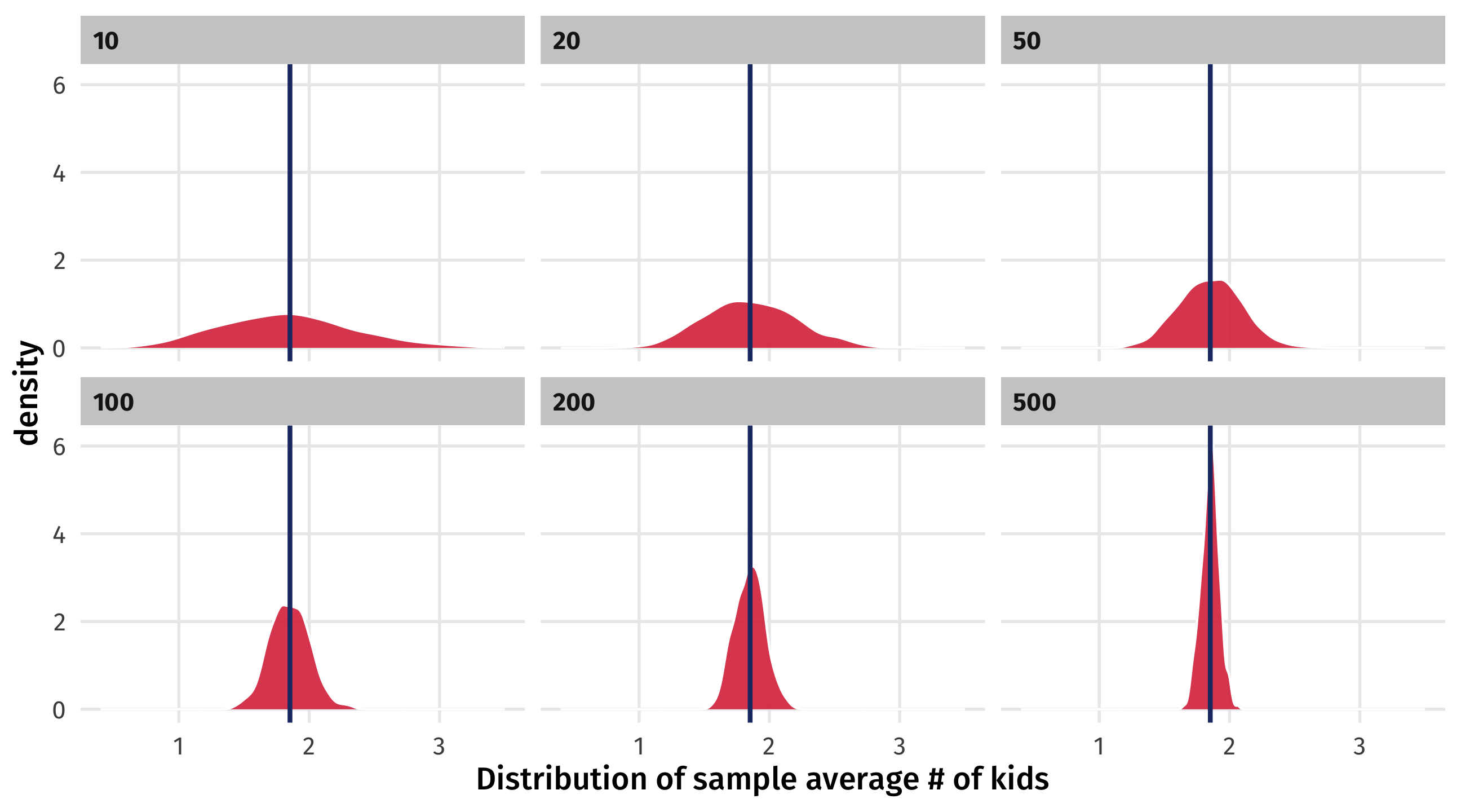
How to simulate
If we take lots of samples of size 20 \(\rightarrow\) uncertainty in a sample of 20
How to simulate
If we take lots of samples of size 100 \(\rightarrow\) uncertainty in a sample of 100
How to simulate
So to see how uncertain we should feel about gss_sm, we should take many samples that are the same size as gss_sm
Note
nrow(DATA) tells you how many observations in data object
Problem
If we have a dataset of 2,867 observations and ask R to randomly pick 2,867 observations, we’ll just get a bunch of copies of the original dataset
Solution: sample with replacement \(\rightarrow\) once we draw an observation it goes back into the dataset, ad can be sampled again
Sampling with replacement
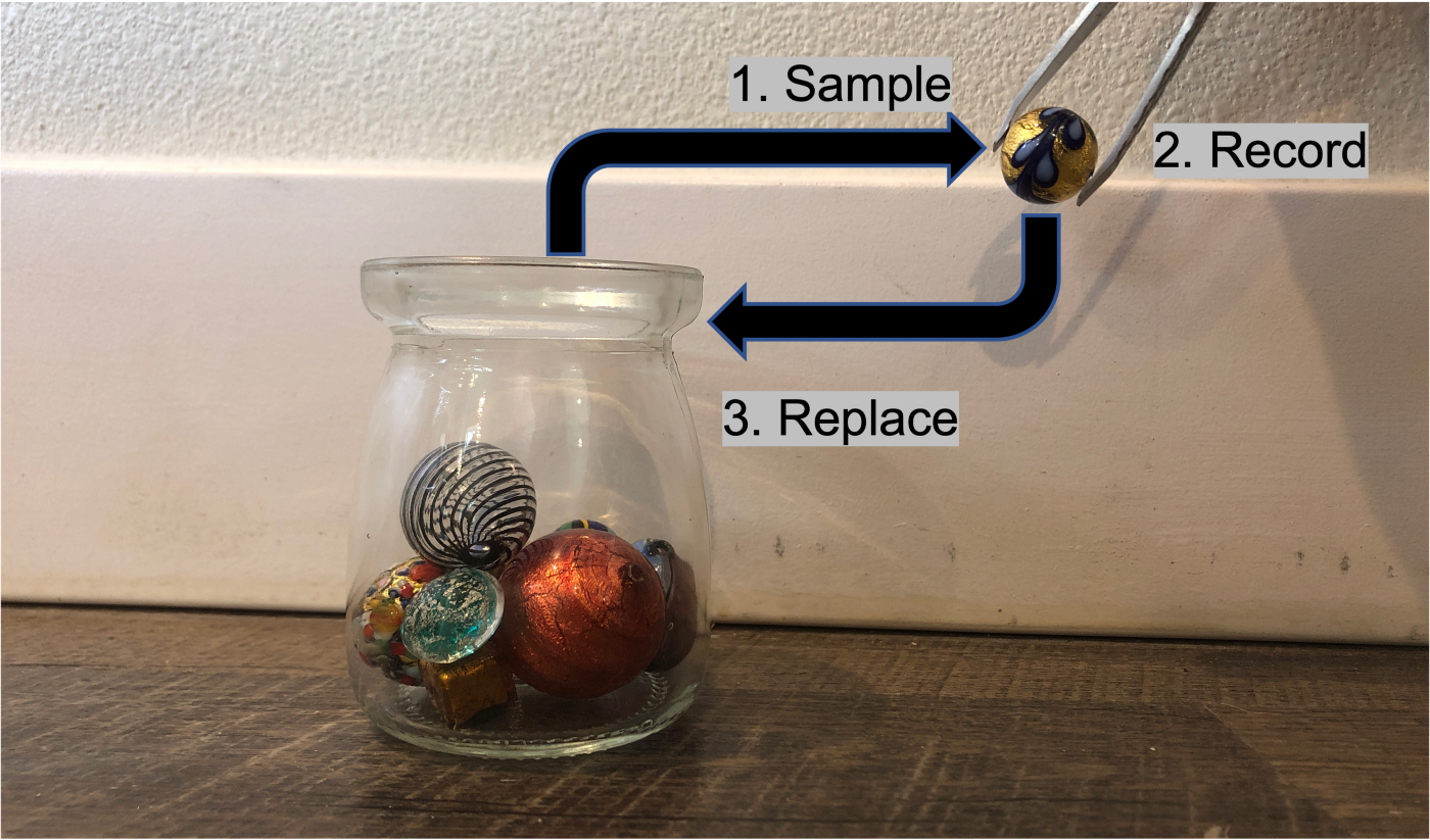
Sampling with and without replacement
If we were sampling 4 of these delicious fruits:
[1] "Mango" "Pineapple" "Banana" "Blackberry"It would look like this, with and without replacement:
| Sample, no replace | Mango | Banana | Pineapple | Blackberry |
| Sample, replace | Pineapple | Pineapple | Banana | Blackberry |
Bootstrapping
- Generating many, same-sized samples with replacement is called bootstrapping
- Replacement lets us generate samples that randomly differ from ours
- Use the distribution of bootstrapped samples to quantify uncertainty

Back to the kids
How uncertain should we be of our estimate of the avg. number of kids in the US, Given that it’s based on our one sample, gss_sm? We can bootstrap:
boot_kids = gss_sm %>%
  rep_sample_n(size = nrow(gss_sm), reps = 1000, replace = TRUE) %>%
  summarise(avg_kids = mean(childs, na.rm = TRUE))
boot_kids| replicate | avg_kids |
| 1 | 1.88 |
| 2 | 1.85 |
| 3 | 1.88 |
| 4 | 1.87 |
| 5 | 1.88 |
| 6 | 1.87 |
| 7 | 1.83 |
| 8 | 1.84 |
| 9 | 1.82 |
| 10 | 1.77 |
| 11 | 1.85 |
| 12 | 1.88 |
| 13 | 1.85 |
| 14 | 1.88 |
| 15 | 1.85 |
| 16 | 1.82 |
| 17 | 1.81 |
| 18 | 1.86 |
| 19 | 1.82 |
| 20 | 1.88 |
| 21 | 1.94 |
| 22 | 1.84 |
| 23 | 1.87 |
| 24 | 1.9 |
| 25 | 1.83 |
| 26 | 1.85 |
| 27 | 1.84 |
| 28 | 1.84 |
| 29 | 1.84 |
| 30 | 1.84 |
| 31 | 1.82 |
| 32 | 1.86 |
| 33 | 1.86 |
| 34 | 1.83 |
| 35 | 1.85 |
| 36 | 1.82 |
| 37 | 1.86 |
| 38 | 1.84 |
| 39 | 1.83 |
| 40 | 1.8 |
| 41 | 1.81 |
| 42 | 1.86 |
| 43 | 1.87 |
| 44 | 1.79 |
| 45 | 1.9 |
| 46 | 1.84 |
| 47 | 1.9 |
| 48 | 1.86 |
| 49 | 1.8 |
| 50 | 1.84 |
| 51 | 1.85 |
| 52 | 1.86 |
| 53 | 1.85 |
| 54 | 1.88 |
| 55 | 1.85 |
| 56 | 1.85 |
| 57 | 1.86 |
| 58 | 1.87 |
| 59 | 1.87 |
| 60 | 1.86 |
| 61 | 1.86 |
| 62 | 1.9 |
| 63 | 1.87 |
| 64 | 1.86 |
| 65 | 1.84 |
| 66 | 1.85 |
| 67 | 1.87 |
| 68 | 1.88 |
| 69 | 1.81 |
| 70 | 1.87 |
| 71 | 1.82 |
| 72 | 1.86 |
| 73 | 1.84 |
| 74 | 1.84 |
| 75 | 1.87 |
| 76 | 1.84 |
| 77 | 1.87 |
| 78 | 1.85 |
| 79 | 1.88 |
| 80 | 1.89 |
| 81 | 1.92 |
| 82 | 1.88 |
| 83 | 1.92 |
| 84 | 1.83 |
| 85 | 1.86 |
| 86 | 1.83 |
| 87 | 1.88 |
| 88 | 1.83 |
| 89 | 1.88 |
| 90 | 1.88 |
| 91 | 1.86 |
| 92 | 1.9 |
| 93 | 1.9 |
| 94 | 1.85 |
| 95 | 1.81 |
| 96 | 1.84 |
| 97 | 1.88 |
| 98 | 1.85 |
| 99 | 1.78 |
| 100 | 1.82 |
| 101 | 1.85 |
| 102 | 1.85 |
| 103 | 1.86 |
| 104 | 1.8 |
| 105 | 1.87 |
| 106 | 1.84 |
| 107 | 1.85 |
| 108 | 1.86 |
| 109 | 1.91 |
| 110 | 1.87 |
| 111 | 1.82 |
| 112 | 1.86 |
| 113 | 1.82 |
| 114 | 1.87 |
| 115 | 1.86 |
| 116 | 1.81 |
| 117 | 1.84 |
| 118 | 1.89 |
| 119 | 1.84 |
| 120 | 1.88 |
| 121 | 1.87 |
| 122 | 1.88 |
| 123 | 1.84 |
| 124 | 1.77 |
| 125 | 1.85 |
| 126 | 1.88 |
| 127 | 1.86 |
| 128 | 1.88 |
| 129 | 1.88 |
| 130 | 1.86 |
| 131 | 1.82 |
| 132 | 1.81 |
| 133 | 1.9 |
| 134 | 1.87 |
| 135 | 1.89 |
| 136 | 1.84 |
| 137 | 1.91 |
| 138 | 1.82 |
| 139 | 1.84 |
| 140 | 1.82 |
| 141 | 1.81 |
| 142 | 1.89 |
| 143 | 1.83 |
| 144 | 1.87 |
| 145 | 1.79 |
| 146 | 1.85 |
| 147 | 1.85 |
| 148 | 1.87 |
| 149 | 1.85 |
| 150 | 1.85 |
| 151 | 1.83 |
| 152 | 1.84 |
| 153 | 1.88 |
| 154 | 1.87 |
| 155 | 1.85 |
| 156 | 1.85 |
| 157 | 1.89 |
| 158 | 1.82 |
| 159 | 1.84 |
| 160 | 1.85 |
| 161 | 1.88 |
| 162 | 1.9 |
| 163 | 1.81 |
| 164 | 1.89 |
| 165 | 1.81 |
| 166 | 1.9 |
| 167 | 1.83 |
| 168 | 1.85 |
| 169 | 1.82 |
| 170 | 1.84 |
| 171 | 1.81 |
| 172 | 1.85 |
| 173 | 1.85 |
| 174 | 1.82 |
| 175 | 1.85 |
| 176 | 1.82 |
| 177 | 1.82 |
| 178 | 1.89 |
| 179 | 1.91 |
| 180 | 1.9 |
| 181 | 1.85 |
| 182 | 1.84 |
| 183 | 1.88 |
| 184 | 1.86 |
| 185 | 1.84 |
| 186 | 1.86 |
| 187 | 1.83 |
| 188 | 1.81 |
| 189 | 1.87 |
| 190 | 1.88 |
| 191 | 1.87 |
| 192 | 1.85 |
| 193 | 1.91 |
| 194 | 1.86 |
| 195 | 1.83 |
| 196 | 1.83 |
| 197 | 1.81 |
| 198 | 1.86 |
| 199 | 1.91 |
| 200 | 1.85 |
| 201 | 1.81 |
| 202 | 1.83 |
| 203 | 1.85 |
| 204 | 1.82 |
| 205 | 1.9 |
| 206 | 1.81 |
| 207 | 1.89 |
| 208 | 1.8 |
| 209 | 1.85 |
| 210 | 1.82 |
| 211 | 1.88 |
| 212 | 1.87 |
| 213 | 1.84 |
| 214 | 1.84 |
| 215 | 1.86 |
| 216 | 1.82 |
| 217 | 1.86 |
| 218 | 1.86 |
| 219 | 1.86 |
| 220 | 1.85 |
| 221 | 1.88 |
| 222 | 1.9 |
| 223 | 1.83 |
| 224 | 1.87 |
| 225 | 1.88 |
| 226 | 1.88 |
| 227 | 1.86 |
| 228 | 1.88 |
| 229 | 1.84 |
| 230 | 1.79 |
| 231 | 1.88 |
| 232 | 1.88 |
| 233 | 1.79 |
| 234 | 1.82 |
| 235 | 1.85 |
| 236 | 1.84 |
| 237 | 1.83 |
| 238 | 1.79 |
| 239 | 1.83 |
| 240 | 1.84 |
| 241 | 1.88 |
| 242 | 1.81 |
| 243 | 1.84 |
| 244 | 1.88 |
| 245 | 1.83 |
| 246 | 1.82 |
| 247 | 1.81 |
| 248 | 1.83 |
| 249 | 1.86 |
| 250 | 1.84 |
| 251 | 1.87 |
| 252 | 1.83 |
| 253 | 1.88 |
| 254 | 1.82 |
| 255 | 1.83 |
| 256 | 1.84 |
| 257 | 1.87 |
| 258 | 1.9 |
| 259 | 1.85 |
| 260 | 1.83 |
| 261 | 1.85 |
| 262 | 1.85 |
| 263 | 1.86 |
| 264 | 1.85 |
| 265 | 1.84 |
| 266 | 1.85 |
| 267 | 1.88 |
| 268 | 1.84 |
| 269 | 1.83 |
| 270 | 1.84 |
| 271 | 1.88 |
| 272 | 1.81 |
| 273 | 1.86 |
| 274 | 1.85 |
| 275 | 1.89 |
| 276 | 1.93 |
| 277 | 1.89 |
| 278 | 1.83 |
| 279 | 1.88 |
| 280 | 1.84 |
| 281 | 1.84 |
| 282 | 1.8 |
| 283 | 1.83 |
| 284 | 1.85 |
| 285 | 1.89 |
| 286 | 1.86 |
| 287 | 1.84 |
| 288 | 1.84 |
| 289 | 1.92 |
| 290 | 1.83 |
| 291 | 1.9 |
| 292 | 1.9 |
| 293 | 1.93 |
| 294 | 1.84 |
| 295 | 1.9 |
| 296 | 1.82 |
| 297 | 1.86 |
| 298 | 1.83 |
| 299 | 1.88 |
| 300 | 1.83 |
| 301 | 1.85 |
| 302 | 1.84 |
| 303 | 1.84 |
| 304 | 1.89 |
| 305 | 1.91 |
| 306 | 1.82 |
| 307 | 1.87 |
| 308 | 1.9 |
| 309 | 1.86 |
| 310 | 1.83 |
| 311 | 1.9 |
| 312 | 1.88 |
| 313 | 1.85 |
| 314 | 1.87 |
| 315 | 1.86 |
| 316 | 1.87 |
| 317 | 1.89 |
| 318 | 1.84 |
| 319 | 1.87 |
| 320 | 1.85 |
| 321 | 1.85 |
| 322 | 1.87 |
| 323 | 1.83 |
| 324 | 1.91 |
| 325 | 1.9 |
| 326 | 1.83 |
| 327 | 1.84 |
| 328 | 1.87 |
| 329 | 1.89 |
| 330 | 1.84 |
| 331 | 1.78 |
| 332 | 1.79 |
| 333 | 1.88 |
| 334 | 1.92 |
| 335 | 1.84 |
| 336 | 1.8 |
| 337 | 1.92 |
| 338 | 1.86 |
| 339 | 1.87 |
| 340 | 1.89 |
| 341 | 1.81 |
| 342 | 1.79 |
| 343 | 1.79 |
| 344 | 1.84 |
| 345 | 1.84 |
| 346 | 1.91 |
| 347 | 1.76 |
| 348 | 1.84 |
| 349 | 1.89 |
| 350 | 1.82 |
| 351 | 1.8 |
| 352 | 1.88 |
| 353 | 1.92 |
| 354 | 1.82 |
| 355 | 1.87 |
| 356 | 1.93 |
| 357 | 1.87 |
| 358 | 1.92 |
| 359 | 1.81 |
| 360 | 1.86 |
| 361 | 1.81 |
| 362 | 1.83 |
| 363 | 1.82 |
| 364 | 1.83 |
| 365 | 1.85 |
| 366 | 1.83 |
| 367 | 1.84 |
| 368 | 1.84 |
| 369 | 1.9 |
| 370 | 1.9 |
| 371 | 1.84 |
| 372 | 1.82 |
| 373 | 1.86 |
| 374 | 1.86 |
| 375 | 1.9 |
| 376 | 1.84 |
| 377 | 1.88 |
| 378 | 1.9 |
| 379 | 1.79 |
| 380 | 1.87 |
| 381 | 1.87 |
| 382 | 1.79 |
| 383 | 1.87 |
| 384 | 1.77 |
| 385 | 1.81 |
| 386 | 1.86 |
| 387 | 1.87 |
| 388 | 1.82 |
| 389 | 1.89 |
| 390 | 1.85 |
| 391 | 1.82 |
| 392 | 1.83 |
| 393 | 1.88 |
| 394 | 1.84 |
| 395 | 1.82 |
| 396 | 1.91 |
| 397 | 1.81 |
| 398 | 1.89 |
| 399 | 1.85 |
| 400 | 1.85 |
| 401 | 1.85 |
| 402 | 1.85 |
| 403 | 1.82 |
| 404 | 1.84 |
| 405 | 1.8 |
| 406 | 1.86 |
| 407 | 1.85 |
| 408 | 1.84 |
| 409 | 1.79 |
| 410 | 1.84 |
| 411 | 1.84 |
| 412 | 1.9 |
| 413 | 1.89 |
| 414 | 1.84 |
| 415 | 1.89 |
| 416 | 1.8 |
| 417 | 1.88 |
| 418 | 1.87 |
| 419 | 1.9 |
| 420 | 1.81 |
| 421 | 1.82 |
| 422 | 1.88 |
| 423 | 1.87 |
| 424 | 1.88 |
| 425 | 1.9 |
| 426 | 1.79 |
| 427 | 1.84 |
| 428 | 1.82 |
| 429 | 1.88 |
| 430 | 1.76 |
| 431 | 1.84 |
| 432 | 1.83 |
| 433 | 1.83 |
| 434 | 1.81 |
| 435 | 1.89 |
| 436 | 1.86 |
| 437 | 1.84 |
| 438 | 1.86 |
| 439 | 1.84 |
| 440 | 1.86 |
| 441 | 1.86 |
| 442 | 1.88 |
| 443 | 1.88 |
| 444 | 1.85 |
| 445 | 1.88 |
| 446 | 1.86 |
| 447 | 1.83 |
| 448 | 1.84 |
| 449 | 1.85 |
| 450 | 1.92 |
| 451 | 1.82 |
| 452 | 1.93 |
| 453 | 1.84 |
| 454 | 1.82 |
| 455 | 1.85 |
| 456 | 1.8 |
| 457 | 1.86 |
| 458 | 1.84 |
| 459 | 1.84 |
| 460 | 1.84 |
| 461 | 1.83 |
| 462 | 1.83 |
| 463 | 1.84 |
| 464 | 1.9 |
| 465 | 1.82 |
| 466 | 1.85 |
| 467 | 1.87 |
| 468 | 1.82 |
| 469 | 1.83 |
| 470 | 1.83 |
| 471 | 1.88 |
| 472 | 1.75 |
| 473 | 1.87 |
| 474 | 1.94 |
| 475 | 1.86 |
| 476 | 1.84 |
| 477 | 1.85 |
| 478 | 1.9 |
| 479 | 1.85 |
| 480 | 1.76 |
| 481 | 1.85 |
| 482 | 1.83 |
| 483 | 1.85 |
| 484 | 1.85 |
| 485 | 1.85 |
| 486 | 1.87 |
| 487 | 1.83 |
| 488 | 1.8 |
| 489 | 1.88 |
| 490 | 1.8 |
| 491 | 1.87 |
| 492 | 1.9 |
| 493 | 1.87 |
| 494 | 1.88 |
| 495 | 1.86 |
| 496 | 1.89 |
| 497 | 1.89 |
| 498 | 1.84 |
| 499 | 1.87 |
| 500 | 1.85 |
| 501 | 1.82 |
| 502 | 1.82 |
| 503 | 1.83 |
| 504 | 1.8 |
| 505 | 1.86 |
| 506 | 1.89 |
| 507 | 1.84 |
| 508 | 1.86 |
| 509 | 1.81 |
| 510 | 1.9 |
| 511 | 1.92 |
| 512 | 1.79 |
| 513 | 1.82 |
| 514 | 1.85 |
| 515 | 1.86 |
| 516 | 1.85 |
| 517 | 1.83 |
| 518 | 1.85 |
| 519 | 1.83 |
| 520 | 1.92 |
| 521 | 1.82 |
| 522 | 1.85 |
| 523 | 1.81 |
| 524 | 1.88 |
| 525 | 1.86 |
| 526 | 1.82 |
| 527 | 1.85 |
| 528 | 1.81 |
| 529 | 1.86 |
| 530 | 1.87 |
| 531 | 1.88 |
| 532 | 1.84 |
| 533 | 1.84 |
| 534 | 1.84 |
| 535 | 1.85 |
| 536 | 1.8 |
| 537 | 1.87 |
| 538 | 1.84 |
| 539 | 1.8 |
| 540 | 1.79 |
| 541 | 1.91 |
| 542 | 1.83 |
| 543 | 1.89 |
| 544 | 1.84 |
| 545 | 1.88 |
| 546 | 1.81 |
| 547 | 1.83 |
| 548 | 1.9 |
| 549 | 1.88 |
| 550 | 1.86 |
| 551 | 1.81 |
| 552 | 1.84 |
| 553 | 1.8 |
| 554 | 1.81 |
| 555 | 1.84 |
| 556 | 1.93 |
| 557 | 1.93 |
| 558 | 1.83 |
| 559 | 1.85 |
| 560 | 1.81 |
| 561 | 1.86 |
| 562 | 1.85 |
| 563 | 1.82 |
| 564 | 1.88 |
| 565 | 1.89 |
| 566 | 1.81 |
| 567 | 1.92 |
| 568 | 1.86 |
| 569 | 1.83 |
| 570 | 1.86 |
| 571 | 1.79 |
| 572 | 1.83 |
| 573 | 1.82 |
| 574 | 1.85 |
| 575 | 1.85 |
| 576 | 1.9 |
| 577 | 1.88 |
| 578 | 1.89 |
| 579 | 1.91 |
| 580 | 1.83 |
| 581 | 1.86 |
| 582 | 1.91 |
| 583 | 1.88 |
| 584 | 1.84 |
| 585 | 1.86 |
| 586 | 1.81 |
| 587 | 1.86 |
| 588 | 1.83 |
| 589 | 1.89 |
| 590 | 1.86 |
| 591 | 1.83 |
| 592 | 1.83 |
| 593 | 1.83 |
| 594 | 1.89 |
| 595 | 1.87 |
| 596 | 1.81 |
| 597 | 1.86 |
| 598 | 1.86 |
| 599 | 1.82 |
| 600 | 1.84 |
| 601 | 1.85 |
| 602 | 1.83 |
| 603 | 1.86 |
| 604 | 1.88 |
| 605 | 1.86 |
| 606 | 1.89 |
| 607 | 1.86 |
| 608 | 1.86 |
| 609 | 1.81 |
| 610 | 1.87 |
| 611 | 1.91 |
| 612 | 1.87 |
| 613 | 1.87 |
| 614 | 1.78 |
| 615 | 1.89 |
| 616 | 1.82 |
| 617 | 1.86 |
| 618 | 1.9 |
| 619 | 1.81 |
| 620 | 1.88 |
| 621 | 1.83 |
| 622 | 1.9 |
| 623 | 1.83 |
| 624 | 1.86 |
| 625 | 1.84 |
| 626 | 1.84 |
| 627 | 1.85 |
| 628 | 1.86 |
| 629 | 1.86 |
| 630 | 1.87 |
| 631 | 1.86 |
| 632 | 1.85 |
| 633 | 1.8 |
| 634 | 1.84 |
| 635 | 1.83 |
| 636 | 1.87 |
| 637 | 1.83 |
| 638 | 1.93 |
| 639 | 1.9 |
| 640 | 1.85 |
| 641 | 1.89 |
| 642 | 1.81 |
| 643 | 1.8 |
| 644 | 1.92 |
| 645 | 1.81 |
| 646 | 1.88 |
| 647 | 1.77 |
| 648 | 1.82 |
| 649 | 1.9 |
| 650 | 1.88 |
| 651 | 1.84 |
| 652 | 1.81 |
| 653 | 1.85 |
| 654 | 1.85 |
| 655 | 1.82 |
| 656 | 1.9 |
| 657 | 1.85 |
| 658 | 1.85 |
| 659 | 1.85 |
| 660 | 1.83 |
| 661 | 1.84 |
| 662 | 1.85 |
| 663 | 1.85 |
| 664 | 1.9 |
| 665 | 1.85 |
| 666 | 1.86 |
| 667 | 1.83 |
| 668 | 1.84 |
| 669 | 1.84 |
| 670 | 1.87 |
| 671 | 1.85 |
| 672 | 1.81 |
| 673 | 1.92 |
| 674 | 1.81 |
| 675 | 1.86 |
| 676 | 1.88 |
| 677 | 1.87 |
| 678 | 1.8 |
| 679 | 1.9 |
| 680 | 1.86 |
| 681 | 1.85 |
| 682 | 1.85 |
| 683 | 1.88 |
| 684 | 1.85 |
| 685 | 1.81 |
| 686 | 1.82 |
| 687 | 1.89 |
| 688 | 1.9 |
| 689 | 1.89 |
| 690 | 1.82 |
| 691 | 1.85 |
| 692 | 1.86 |
| 693 | 1.88 |
| 694 | 1.89 |
| 695 | 1.85 |
| 696 | 1.84 |
| 697 | 1.84 |
| 698 | 1.93 |
| 699 | 1.88 |
| 700 | 1.88 |
| 701 | 1.83 |
| 702 | 1.84 |
| 703 | 1.85 |
| 704 | 1.83 |
| 705 | 1.89 |
| 706 | 1.83 |
| 707 | 1.82 |
| 708 | 1.89 |
| 709 | 1.83 |
| 710 | 1.85 |
| 711 | 1.85 |
| 712 | 1.86 |
| 713 | 1.85 |
| 714 | 1.82 |
| 715 | 1.86 |
| 716 | 1.84 |
| 717 | 1.86 |
| 718 | 1.86 |
| 719 | 1.86 |
| 720 | 1.88 |
| 721 | 1.79 |
| 722 | 1.84 |
| 723 | 1.85 |
| 724 | 1.84 |
| 725 | 1.86 |
| 726 | 1.8 |
| 727 | 1.8 |
| 728 | 1.85 |
| 729 | 1.87 |
| 730 | 1.82 |
| 731 | 1.81 |
| 732 | 1.84 |
| 733 | 1.84 |
| 734 | 1.84 |
| 735 | 1.88 |
| 736 | 1.92 |
| 737 | 1.8 |
| 738 | 1.85 |
| 739 | 1.88 |
| 740 | 1.87 |
| 741 | 1.89 |
| 742 | 1.89 |
| 743 | 1.85 |
| 744 | 1.84 |
| 745 | 1.83 |
| 746 | 1.88 |
| 747 | 1.91 |
| 748 | 1.83 |
| 749 | 1.83 |
| 750 | 1.88 |
| 751 | 1.85 |
| 752 | 1.84 |
| 753 | 1.9 |
| 754 | 1.87 |
| 755 | 1.83 |
| 756 | 1.85 |
| 757 | 1.89 |
| 758 | 1.81 |
| 759 | 1.9 |
| 760 | 1.88 |
| 761 | 1.88 |
| 762 | 1.85 |
| 763 | 1.9 |
| 764 | 1.87 |
| 765 | 1.9 |
| 766 | 1.88 |
| 767 | 1.81 |
| 768 | 1.85 |
| 769 | 1.88 |
| 770 | 1.83 |
| 771 | 1.83 |
| 772 | 1.84 |
| 773 | 1.87 |
| 774 | 1.92 |
| 775 | 1.82 |
| 776 | 1.86 |
| 777 | 1.84 |
| 778 | 1.86 |
| 779 | 1.82 |
| 780 | 1.9 |
| 781 | 1.85 |
| 782 | 1.81 |
| 783 | 1.83 |
| 784 | 1.85 |
| 785 | 1.83 |
| 786 | 1.86 |
| 787 | 1.85 |
| 788 | 1.81 |
| 789 | 1.84 |
| 790 | 1.92 |
| 791 | 1.83 |
| 792 | 1.88 |
| 793 | 1.87 |
| 794 | 1.89 |
| 795 | 1.83 |
| 796 | 1.83 |
| 797 | 1.92 |
| 798 | 1.9 |
| 799 | 1.84 |
| 800 | 1.84 |
| 801 | 1.83 |
| 802 | 1.83 |
| 803 | 1.83 |
| 804 | 1.85 |
| 805 | 1.8 |
| 806 | 1.82 |
| 807 | 1.84 |
| 808 | 1.83 |
| 809 | 1.88 |
| 810 | 1.85 |
| 811 | 1.81 |
| 812 | 1.85 |
| 813 | 1.84 |
| 814 | 1.85 |
| 815 | 1.82 |
| 816 | 1.84 |
| 817 | 1.85 |
| 818 | 1.86 |
| 819 | 1.85 |
| 820 | 1.83 |
| 821 | 1.81 |
| 822 | 1.84 |
| 823 | 1.89 |
| 824 | 1.85 |
| 825 | 1.79 |
| 826 | 1.9 |
| 827 | 1.85 |
| 828 | 1.86 |
| 829 | 1.85 |
| 830 | 1.88 |
| 831 | 1.86 |
| 832 | 1.84 |
| 833 | 1.83 |
| 834 | 1.83 |
| 835 | 1.86 |
| 836 | 1.88 |
| 837 | 1.85 |
| 838 | 1.8 |
| 839 | 1.84 |
| 840 | 1.88 |
| 841 | 1.85 |
| 842 | 1.83 |
| 843 | 1.85 |
| 844 | 1.85 |
| 845 | 1.83 |
| 846 | 1.84 |
| 847 | 1.86 |
| 848 | 1.84 |
| 849 | 1.82 |
| 850 | 1.86 |
| 851 | 1.94 |
| 852 | 1.8 |
| 853 | 1.85 |
| 854 | 1.85 |
| 855 | 1.84 |
| 856 | 1.81 |
| 857 | 1.88 |
| 858 | 1.86 |
| 859 | 1.81 |
| 860 | 1.81 |
| 861 | 1.86 |
| 862 | 1.79 |
| 863 | 1.81 |
| 864 | 1.79 |
| 865 | 1.9 |
| 866 | 1.82 |
| 867 | 1.83 |
| 868 | 1.84 |
| 869 | 1.9 |
| 870 | 1.89 |
| 871 | 1.86 |
| 872 | 1.85 |
| 873 | 1.85 |
| 874 | 1.84 |
| 875 | 1.82 |
| 876 | 1.86 |
| 877 | 1.84 |
| 878 | 1.85 |
| 879 | 1.83 |
| 880 | 1.81 |
| 881 | 1.86 |
| 882 | 1.9 |
| 883 | 1.79 |
| 884 | 1.79 |
| 885 | 1.86 |
| 886 | 1.82 |
| 887 | 1.86 |
| 888 | 1.83 |
| 889 | 1.8 |
| 890 | 1.83 |
| 891 | 1.89 |
| 892 | 1.84 |
| 893 | 1.82 |
| 894 | 1.86 |
| 895 | 1.83 |
| 896 | 1.89 |
| 897 | 1.8 |
| 898 | 1.87 |
| 899 | 1.86 |
| 900 | 1.87 |
| 901 | 1.83 |
| 902 | 1.85 |
| 903 | 1.78 |
| 904 | 1.8 |
| 905 | 1.84 |
| 906 | 1.86 |
| 907 | 1.85 |
| 908 | 1.85 |
| 909 | 1.83 |
| 910 | 1.88 |
| 911 | 1.83 |
| 912 | 1.84 |
| 913 | 1.86 |
| 914 | 1.86 |
| 915 | 1.82 |
| 916 | 1.87 |
| 917 | 1.82 |
| 918 | 1.88 |
| 919 | 1.81 |
| 920 | 1.87 |
| 921 | 1.77 |
| 922 | 1.83 |
| 923 | 1.85 |
| 924 | 1.85 |
| 925 | 1.81 |
| 926 | 1.9 |
| 927 | 1.89 |
| 928 | 1.87 |
| 929 | 1.81 |
| 930 | 1.81 |
| 931 | 1.84 |
| 932 | 1.87 |
| 933 | 1.86 |
| 934 | 1.82 |
| 935 | 1.87 |
| 936 | 1.81 |
| 937 | 1.87 |
| 938 | 1.82 |
| 939 | 1.88 |
| 940 | 1.87 |
| 941 | 1.89 |
| 942 | 1.85 |
| 943 | 1.86 |
| 944 | 1.82 |
| 945 | 1.82 |
| 946 | 1.8 |
| 947 | 1.83 |
| 948 | 1.82 |
| 949 | 1.83 |
| 950 | 1.78 |
| 951 | 1.86 |
| 952 | 1.9 |
| 953 | 1.87 |
| 954 | 1.82 |
| 955 | 1.81 |
| 956 | 1.9 |
| 957 | 1.84 |
| 958 | 1.89 |
| 959 | 1.88 |
| 960 | 1.83 |
| 961 | 1.81 |
| 962 | 1.85 |
| 963 | 1.86 |
| 964 | 1.86 |
| 965 | 1.84 |
| 966 | 1.84 |
| 967 | 1.83 |
| 968 | 1.89 |
| 969 | 1.85 |
| 970 | 1.87 |
| 971 | 1.81 |
| 972 | 1.8 |
| 973 | 1.85 |
| 974 | 1.83 |
| 975 | 1.9 |
| 976 | 1.83 |
| 977 | 1.87 |
| 978 | 1.86 |
| 979 | 1.85 |
| 980 | 1.83 |
| 981 | 1.9 |
| 982 | 1.79 |
| 983 | 1.88 |
| 984 | 1.81 |
| 985 | 1.8 |
| 986 | 1.91 |
| 987 | 1.89 |
| 988 | 1.88 |
| 989 | 1.89 |
| 990 | 1.89 |
| 991 | 1.8 |
| 992 | 1.85 |
| 993 | 1.85 |
| 994 | 1.83 |
| 995 | 1.9 |
| 996 | 1.84 |
| 997 | 1.87 |
| 998 | 1.84 |
| 999 | 1.83 |
| 1000 | 1.86 |
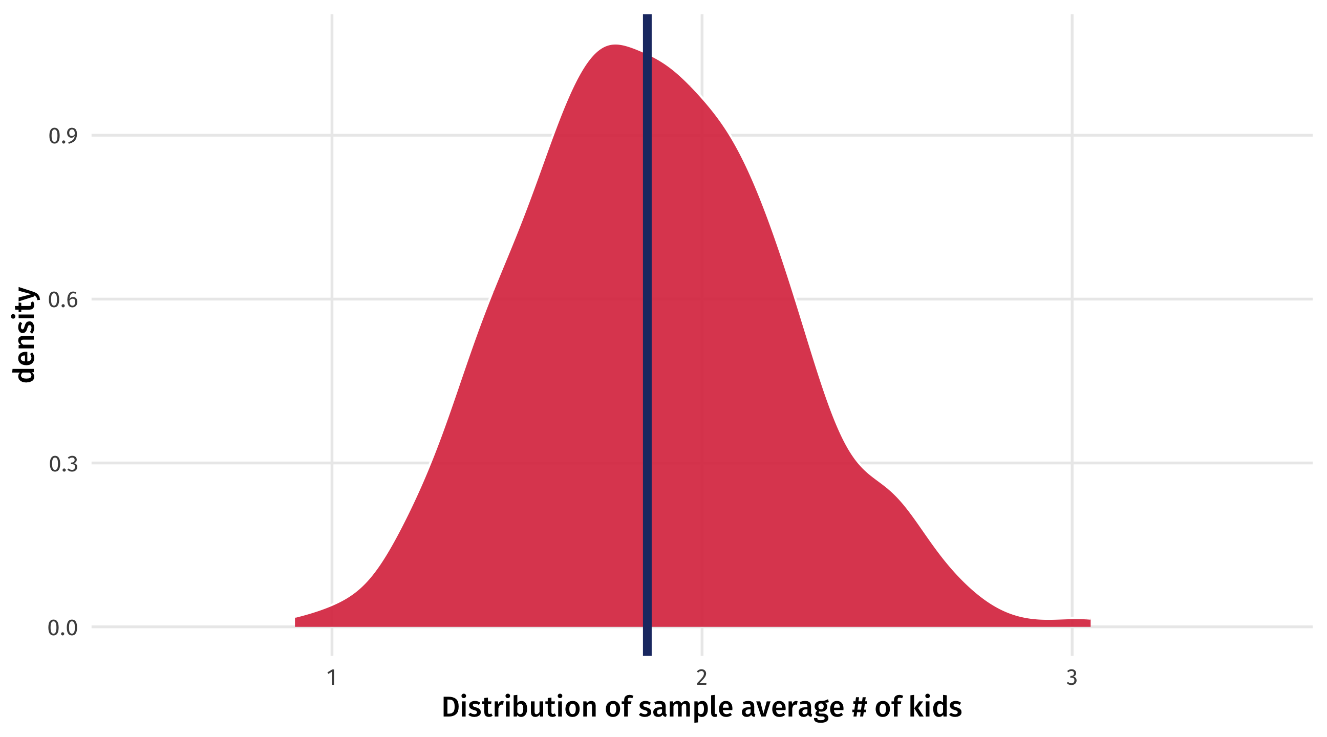
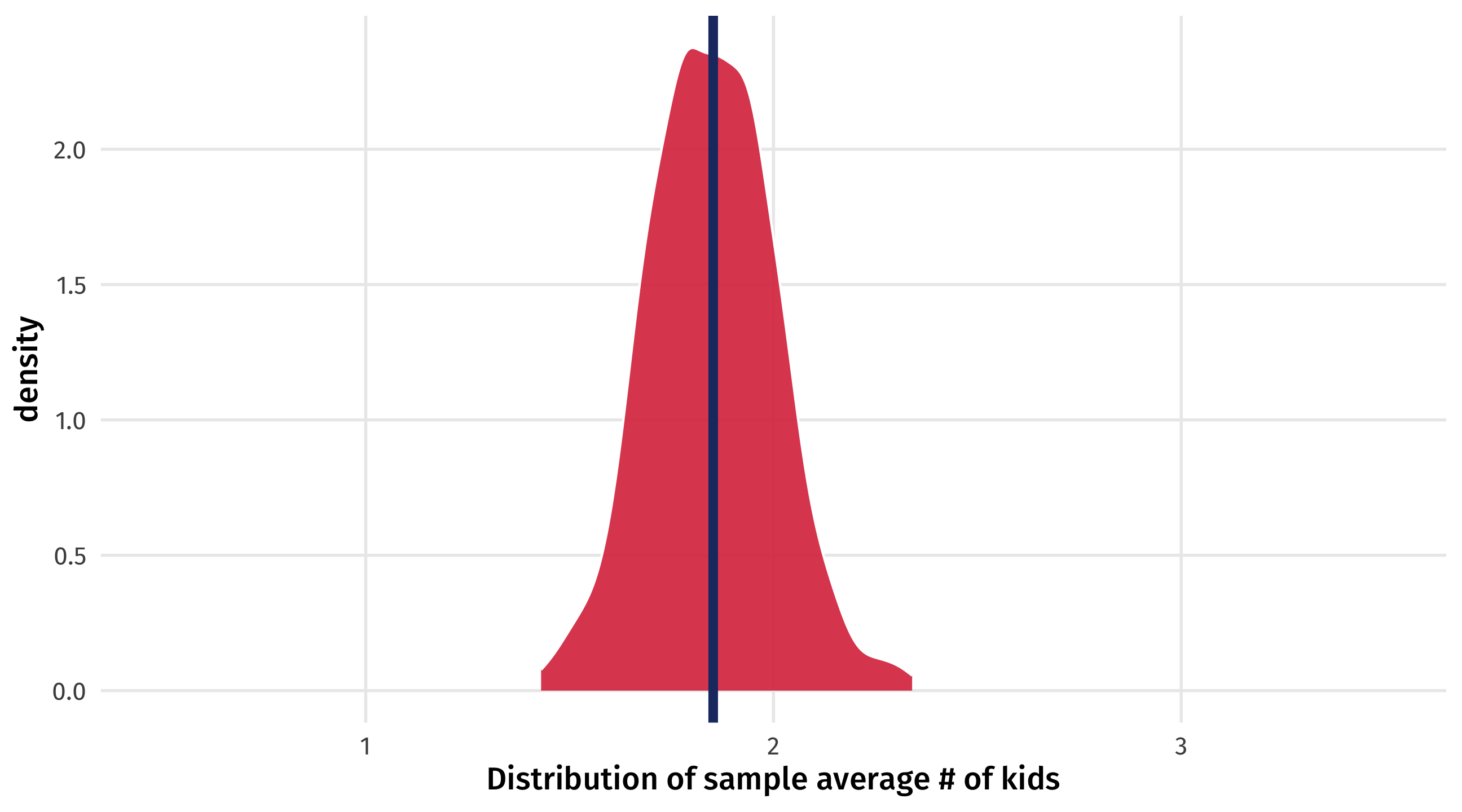
The distribution of bootstrapped estimates
Our estimate and how much simulated estimates might vary across bootstrapped samples that look like ours
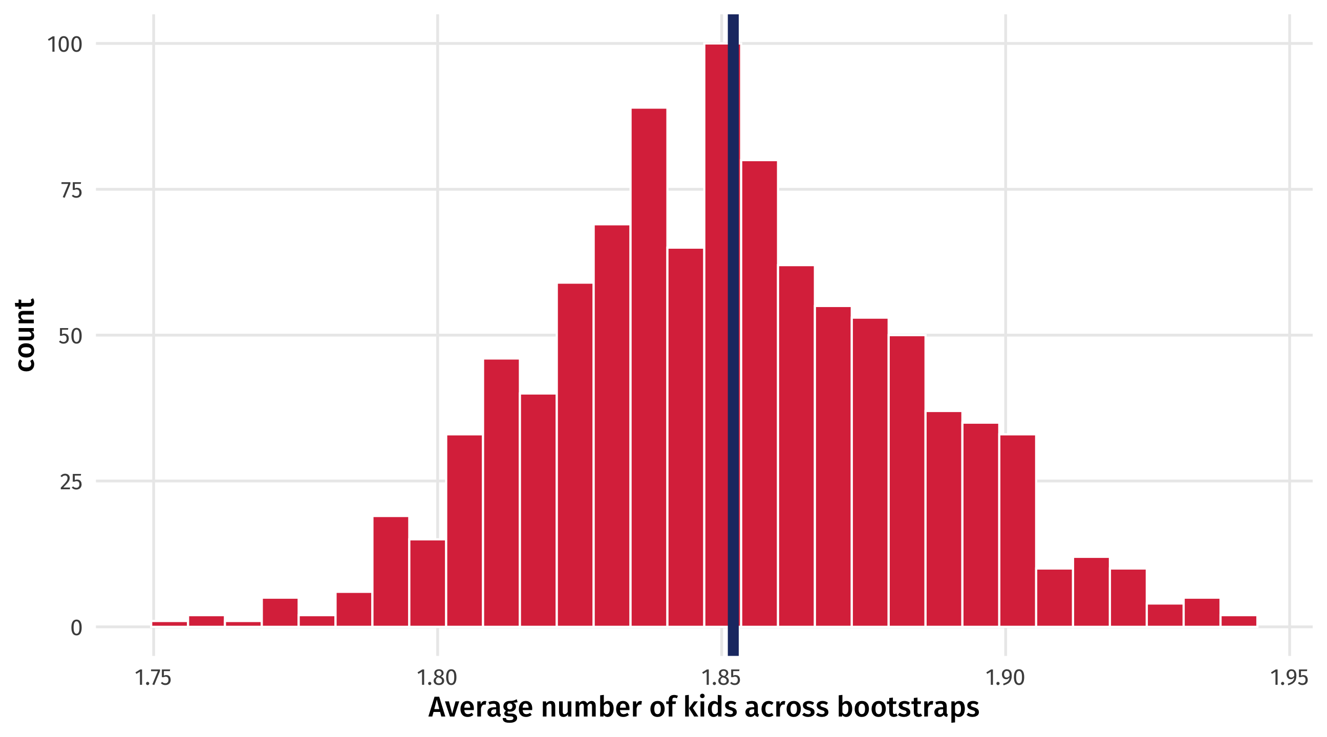
The red is the distribution of bootstrapped sample estimates \(\rightarrow\) the sampling distribution
Quantifying uncertainty
How to quantify uncertainty?
The red histogram is nice, but how can we communicate uncertainty in our estimates in a pithy, more comparable way?
Three approaches:
- The standard error
- The confidence interval
- Statistical significance

The standard error
One way to quantify uncertainty would be to measure how “wide” the distribution of bootstrapped sample estimates is
As we learned so long ago, one way to measure the “spread” of a distribution (i.e., how much a variable varies), is with the standard deviation
The standard deviation of the sampling distribution is called the standard error, or the margin of error
Standard error
This is what you see in the news – that +/- polling/margin of error

Varying uncertainty
As our sample size increases, the standard error decreases
| Sample size | Average (truth = 10) | Standard error |
|---|---|---|
| 10.00 | 9.12 | 0.74 |
| 64.44 | 10.06 | 0.28 |
| 118.89 | 10.11 | 0.19 |
| 173.33 | 10.07 | 0.16 |
| 227.78 | 9.89 | 0.13 |
| 282.22 | 9.94 | 0.12 |
| 336.67 | 10.00 | 0.11 |
| 391.11 | 10.08 | 0.10 |
| 445.56 | 9.99 | 0.09 |
| 500.00 | 9.92 | 0.09 |
The confidence interval
The confidence interval
Another way to quantify uncertainty is to look where most estimates fall
this is the confidence interval: our “best guess” of what we’re trying to estimate
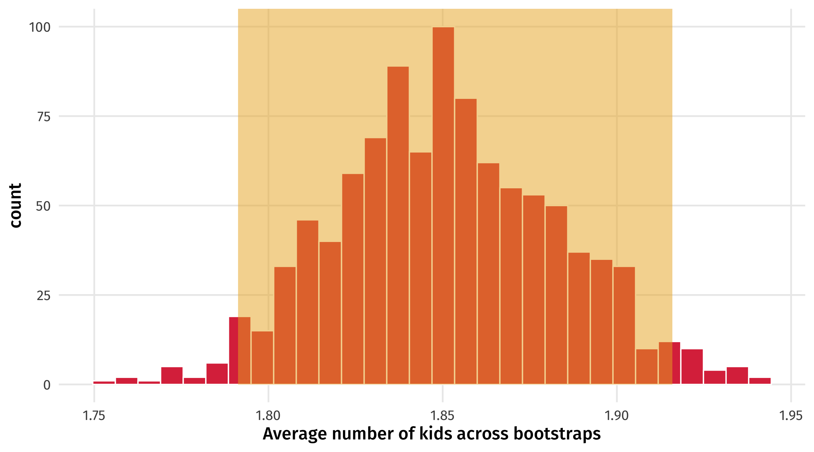
How big to make the interval?
You could report (for example) where the middle 50% of bootstraps fall, or (for example) where the middle 95% of bootstraps fall, but there are tradeoffs!

The tradeoff
You are 50% “confident” that avg. number of kids could vary between 1.83 and 1.87. Narrower range! But low confidence!
You are 95% “confident” that avg. number of kids could vary between 1.79 and 1.92. Higher range! But higher confidence!
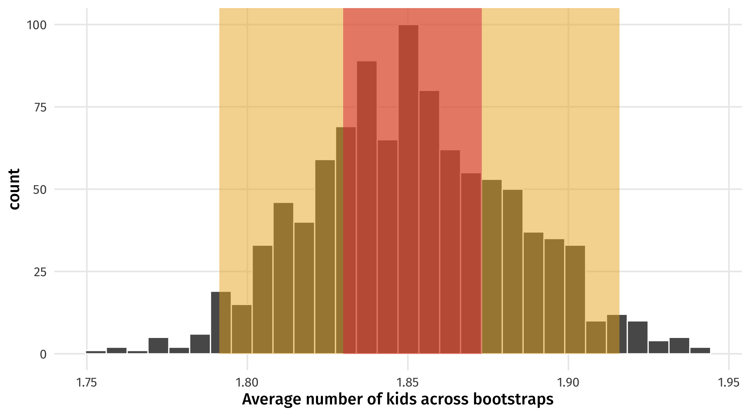
How big to make the interval?
Convention is to look at the middle 95% of the distribution
Where do the middle 95% of the bootstrap estimates fall?
We can use the quantile() function to get here
The 95% confidence confidence interval for the average number of kids in the US is: (1.80, 1.91)
Mirrors of one another
The standard error and confidence interval are actually telling you the same thing
A 95% confidence interval is roughly equal to the Estimate +/- 1.96 \(\times\) standard error
🚨 Your turn: polling the death penalty 🚨
Use the issues data, and:
Pick a state of your choosing. What proportion of respondents support the death penalty in that state?
OK, but how certain are you of that? Generate 1,000 bootstraps and plot the distribution.
Calculate the standard error and the 95% confidence interval of your best guess. Convince yourself the two can be made equivalent.
10:00