Uncertainty I

POL51

Juan F. Tellez

University of California, Davis

December 5, 2023

Plan for today

Why are we uncertain?

Sampling

Good and bad samples

Where things stand

So far: worrying about causality

how can we know the effect of X on Y is not being confounded by something else?

Last bit: how confident are we in our estimates given…

that our estimates are based on samples?

Uncertainty in the wild

The “bounds” in geom_smooth tells us something about how confident we should be in the line:

Uncertainty

Polling error, margin of error, uncertainty bounds, all help to quantify how uncertain we feel about an estimate

Vague sense that we are uncertain about what we are estimating

But why are we uncertain? And how can uncertainty be quantified?

Why are we uncertain?

We don’t have all the data we care about
We have a sample, such as a survey, or a poll, of a population
Problem each sample will look different, and give us a different answer to the question we are trying to answer

What’s going on here? terminology

Term	Meaning	Example
Population	All of the instances of the thing we care about	American adults
Population parameter	The thing about the population we want to know	Average number of kids among American adults
Sample	A subset of the population	A survey
Sample estimate	Our estimate of the population parameter	Average number of kids in survey

Boring example: kids

How many children does the average American adult have? (Population parameter)

Let’s pretend there were only 2,867 people living in the USA, and they were all perfectly sampled in gss_sm

A few rows from gss_sm
year	age	childs	degree	race	sex
2016	71	4	Junior College	White	Male
2016	79	4	High School	Other	Female
2016	53	5	Lt High School	Other	Female
2016	42	4	High School	White	Male
2016	36	2	High School	White	Female

Boring example: kids

How many children does the average American adult have?

We can get the exact answer, since there are only 2,867 Americans, and they’re all in our data:

gss_sm %>% 
  summarise(avg_kids = mean(childs, na.rm = TRUE))

# A tibble: 1 × 1
  avg_kids
     <dbl>
1     1.85

The true average number of children in the US is 1.85 (Population parameter)

Sampling

Now imagine that instead of having data on every American, we only have a sample of 10 Americans

Why do we have a sample? Because interviewing every American is prohibitively costly

Same way a poll works: a sample to estimate American public opinion

Sampling

We can pick one sample of 10 people from gss_sm using the rep_sample_n() function from moderndive:

gss_sm %>% rep_sample_n(size = 10, reps = 1)

# A tibble: 10 × 33
# Groups:   replicate [1]
   replicate  year    id ballot       age childs sibs  degree race  sex   region
       <int> <dbl> <dbl> <labelled> <dbl>  <dbl> <lab> <fct>  <fct> <fct> <fct> 
 1         1  2016   789 3             51      5 0     High … Black Male  South…
 2         1  2016  1530 3             47      0 3     Gradu… White Male  New E…
 3         1  2016   846 2             23      0 6     Junio… Black Fema… E. No…
 4         1  2016   104 3             89      2 3     High … White Fema… Middl…
 5         1  2016   823 3             63      1 9     Lt Hi… Black Fema… E. No…
 6         1  2016  2040 2             78      0 1     High … White Fema… E. No…
 7         1  2016  1837 2             61      3 3     High … White Male  South…
 8         1  2016  2820 3             57      3 2     Junio… White Fema… South…
 9         1  2016  1864 2             62      2 1     High … Black Fema… E. So…
10         1  2016  2159 2             71      2 2     Junio… White Male  W. No…
# ℹ 22 more variables: income16 <fct>, relig <fct>, marital <fct>, padeg <fct>,
#   madeg <fct>, partyid <fct>, polviews <fct>, happy <fct>, partners <fct>,
#   grass <fct>, zodiac <fct>, pres12 <labelled>, wtssall <dbl>,
#   income_rc <fct>, agegrp <fct>, ageq <fct>, siblings <fct>, kids <fct>,
#   religion <fct>, bigregion <fct>, partners_rc <fct>, obama <dbl>

Note

size = size of the sample; reps = number of samples

Sample estimate

We can then calculate the average number of kids among that sample of 10 people

gss_sm %>% rep_sample_n(size = 10, reps = 1) %>% 
  summarise(avg_kids = mean(childs, na.rm = TRUE))

# A tibble: 1 × 2
  replicate avg_kids
      <int>    <dbl>
1         1      2.5

this is our sample estimate of the population parameter

Notice that it does not equal the true population parameter (1.87)

The trouble with samples

Problem: each sample will give you a different estimate. Instead of taking 1 sample of size 10, let’s take 1,000 samples of size 10:

kids_10 = gss_sm %>% rep_sample_n(size = 10, reps = 1000) %>% 
  summarise(avg_kids = mean(childs, na.rm = TRUE))
kids_10

# A tibble: 1,000 × 2
   replicate avg_kids
       <int>    <dbl>
 1         1      2.1
 2         2      1.6
 3         3      1  
 4         4      2.3
 5         5      1.1
 6         6      1.5
 7         7      1.3
 8         8      1.7
 9         9      1.3
10        10      1.2
# ℹ 990 more rows

The trouble with samples

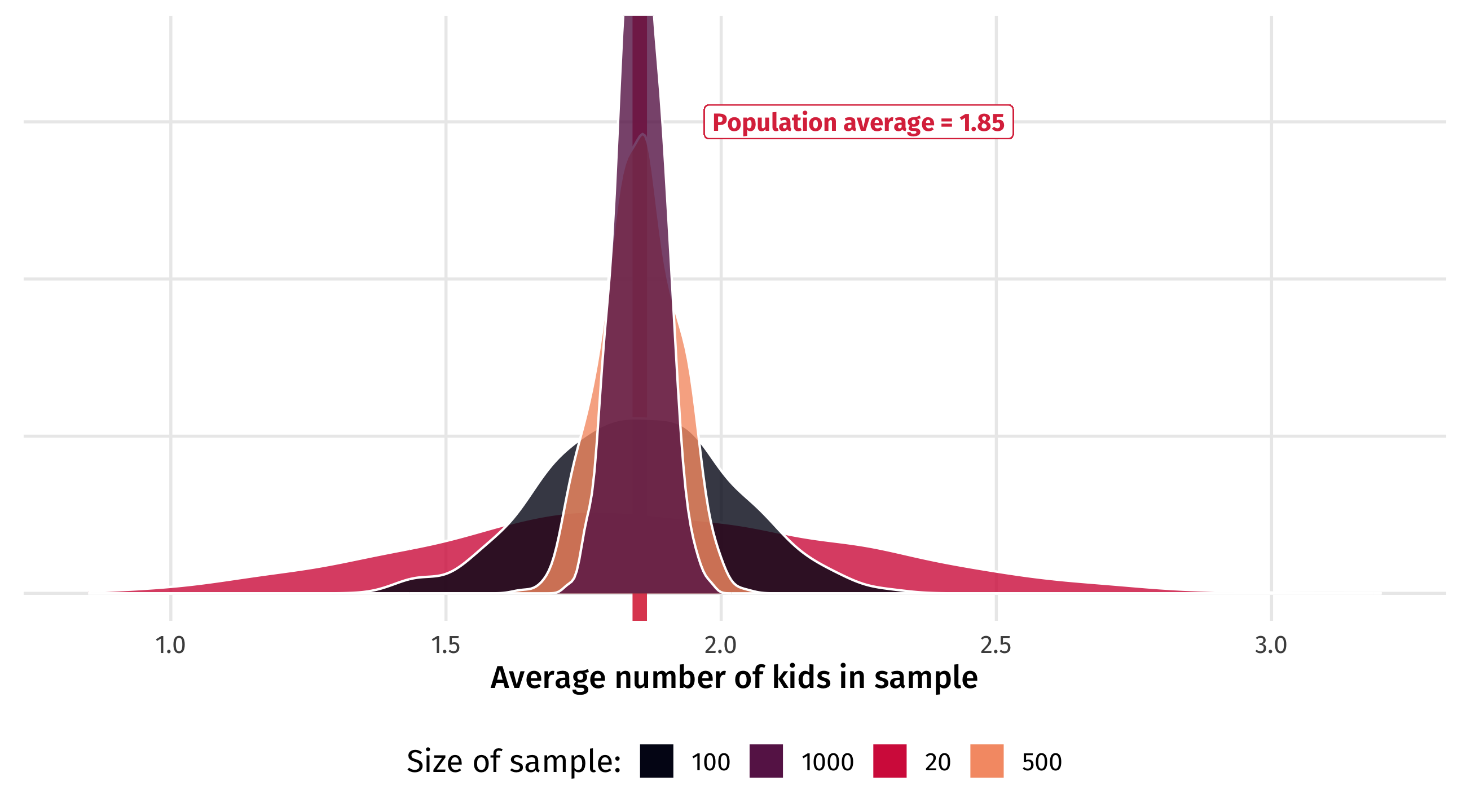
Across 1,000 samples of 10 people each, the estimated average number of kids can vary between 0.4 and 4!! Remember, the true average is 1.85

🚨 Your turn: Views on abortion 🚨

Pretend the gss_abortion dataset from stevedata captures how every American feels about abortion:

Find the average level of support for one of the abortion questions.
Now, take 1,000 samples each of size 10 and calculate the average for each sample. How much do your estimates vary from sample to sample? What’s the min/max?
Plot your sample estimates as a geom_histogram or geom_density.

10:00

Why are we uncertain?

We only ever have a sample (10 random Americans), but we’re interested in something bigger: a population (the whole of gss_sm)

Polls often ask a couple thousand people (if that!), and try to infer something bigger (how all Americans feel about the President)

The problem: Each sample is going to give us different results!

Especially worrisome: some estimates will be way off, totally by chance

A problem for regression

This is also a problem for regression, since every regression estimate is based on a sample

What’s the relationship between sex and vote choice among American voters?

mod1 = lm(obama ~ sex, data = gss_sm)
tidy(mod1)

# A tibble: 2 × 5
  term        estimate std.error statistic   p.value
  <chr>          <dbl>     <dbl>     <dbl>     <dbl>
1 (Intercept)   0.576     0.0177     32.6  5.84e-182
2 sexFemale     0.0871    0.0234      3.72 2.06e-  4

So females were 8.7 percent more likely to vote for Obama than males

This is the population parameter, since we’re pretending all Americans are in gss_sm

Regression estimates vary too

Each sample will produce different regression estimates

replicate	term	estimate
1	sexFemale	-0.44
2	sexFemale	-0.23
3	sexFemale	0.02
4	sexFemale	0.05
5	sexFemale	0.65
6	sexFemale	0.20
7	sexFemale	0.47
8	sexFemale	0.25

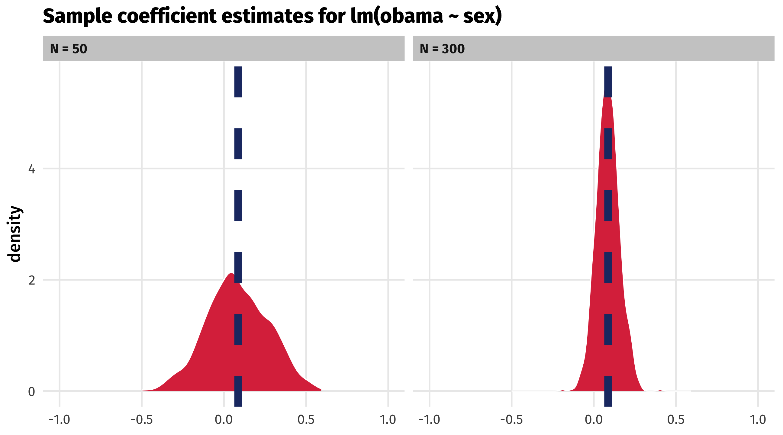
Wrong effect estimates

Many of the effects we estimate below are even negative! This is the opposite of the population parameter (0.087)

The solution

So how do we know if our sample estimate is close to the population parameter?
Turns out that if a sample is random, representative, and large…
…then the LAW OF LARGE NUMBERS tells us that…
the sample estimate will be pretty close to the population parameter

Law of large numbers

With a small sample, estimates can vary a lot:

Law of large numbers

As the sample size (N) increases, estimates begin to converge:

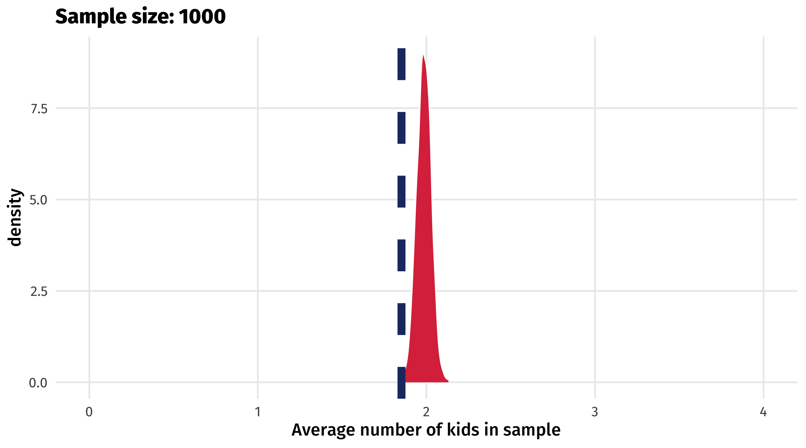
Law of large numbers

They become more concentrated around the population average…

Law of large numbers

And eventually it becomes very unlikely the sample estimate is way off

This works for regression estimates, too

Regression estimates also become more precise as sample size increases:

What’s going on?

The larger our sample, the less likely it is that our estimate (average number of kids, the effect of sex on vote choice, etc.) is way off

This is because as sample size increases, sample estimates tend to converge on the population parameter

Next time = we’ll see how to quantify uncertainty based on this tendency

Intuitive = the more data we have, the less uncertain we should feel

But this only works if we have a good sample

Good and bad samples

There are good and bad samples in the world

Good sample representative of the population and unbiased

Bad sample the opposite of a good sample

What does this mean?

When sampling goes wrong

Imagine that in our quest to find out how many kids the average American has, we do telephone surveys

Younger people are less likely to have a landline than older people, so few young people make it onto our survey

what happens to our estimate?

When sampling goes wrong

We can simulate this by again pretending gss_sm is the whole of the US

Let’s imagine the extreme scenario where no one under 25 makes it into the survey:

gss_sm %>% 
  filter(age >= 25) %>%
  rep_sample_n(size = 10, reps = 1000) %>% 
  summarise(avg_kids = mean(childs, na.rm = TRUE))

I’ve filtered out all people in gss_sm under 25 so they cannot be sampled

When sampling goes wrong

As sample size increases, variability of estimates will still decrease

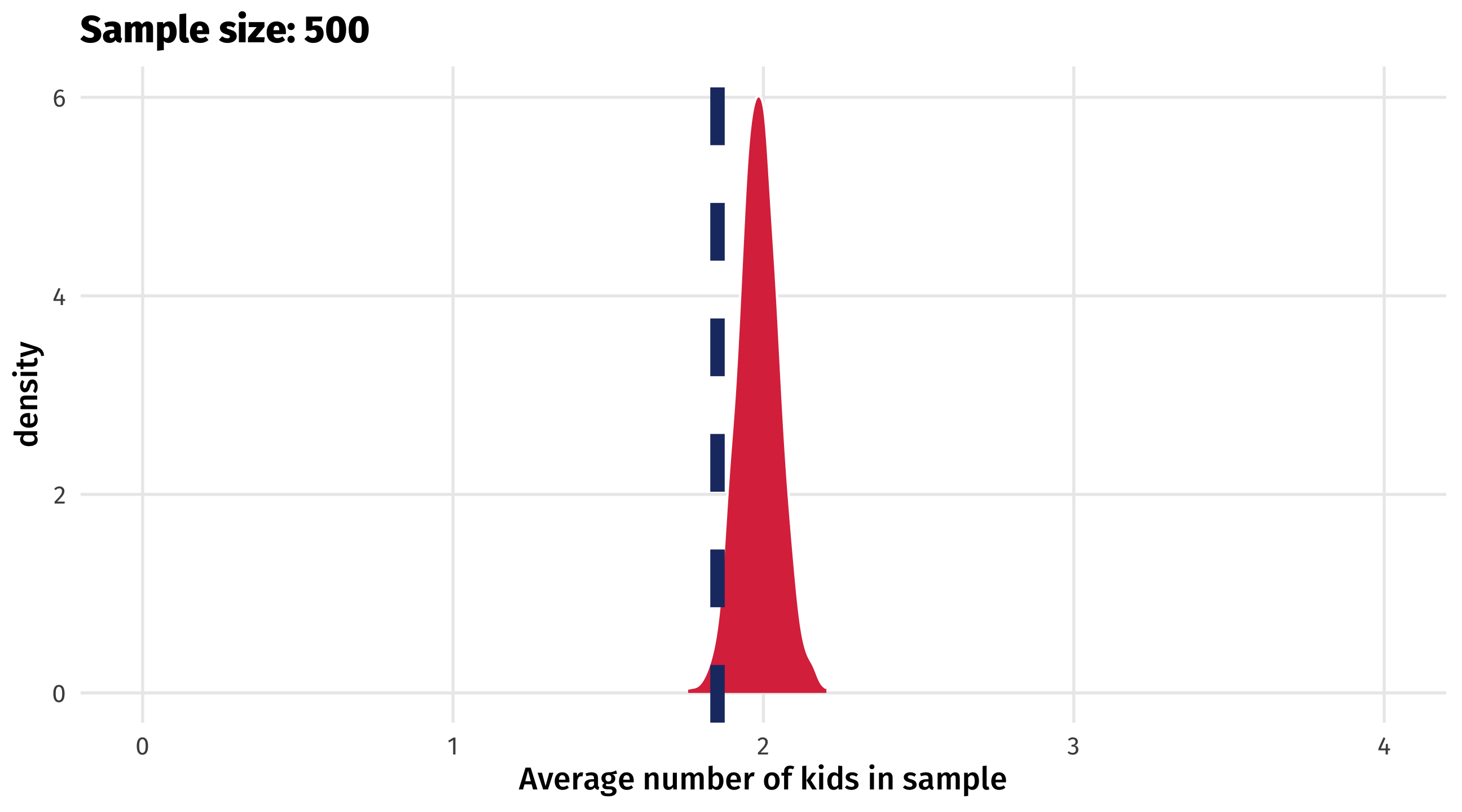
When sampling goes wrong

But estimates will be biased, regardless of sample size

What’s going on?

The sample is not representative of the population (the young people are missing)

This biases our estimate of the population parameter

Randomness is key = everyone needs a similar chance of ending up in the sample

When young people don’t have land-lines, not everyone has a similar chance of ending up in the sample

A big problem!

🚨 Your turn: bias the polls 🚨

Using the gss_abortion data again, imagine you are an evil pollster:

Think about who you would have to exclude from the data to create estimates that benefit the pro-choice and pro-life side of the abortion debate.
Show that even as the sample size increases and estimate variability decreases, we still get biased results.

10:00

Key takeaways

We worry that each sample will give us a different answer, and some answers will be very wrong
The tendency for sample estimates to approach the population parameter as sample size increases (the law of large numbers) saves us
But it all depends on whether we have a random, representative (good) sample; no amount of data in the world will correct for sampling bias