
Modeling I
POL51
September 30, 2024
Patterns and correlations

A useful way to talk about these patterns is in terms of correlations
When we see a pattern between two (or more) variables, we say they are correlated; when we don’t see one, we say they are uncorrelated
Correlations can be strong or weak, positive or negative
Correlations: strength
When two variables “move together”, the correlation is strong
When they don’t “move together”, the correlation is weak

Correlations: strength
Better heuristic: knowing about one variable tells you something about the other
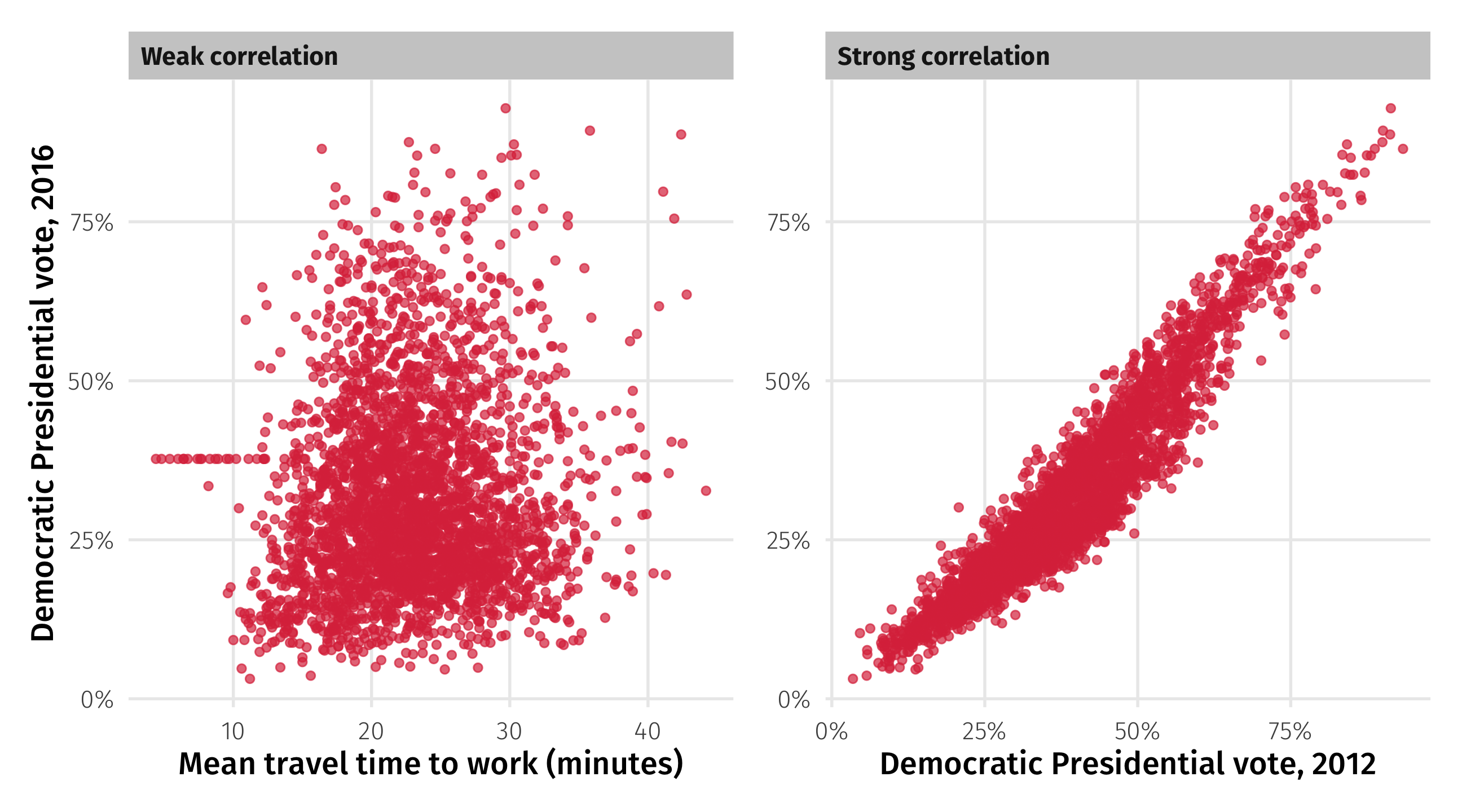
Strong: if you know how a county voted in 2012, you have a good guess for 2016
Weak: if you know a county’s average commute time, you know almost nothing about how it votes
Correlation: strength
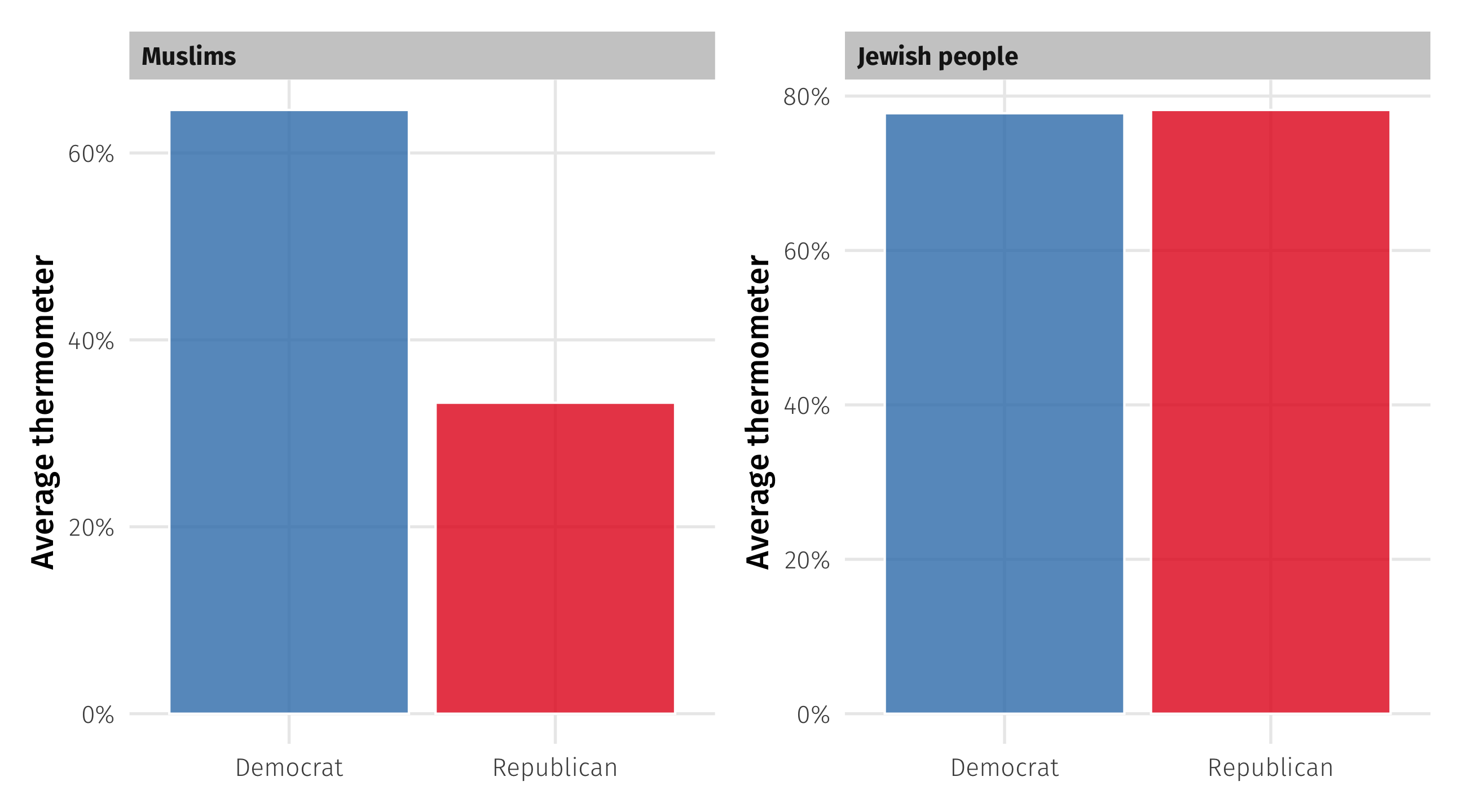
We also talk (informally) about correlations that include categorical variables
Big gaps between groups \(\rightarrow\) correlated
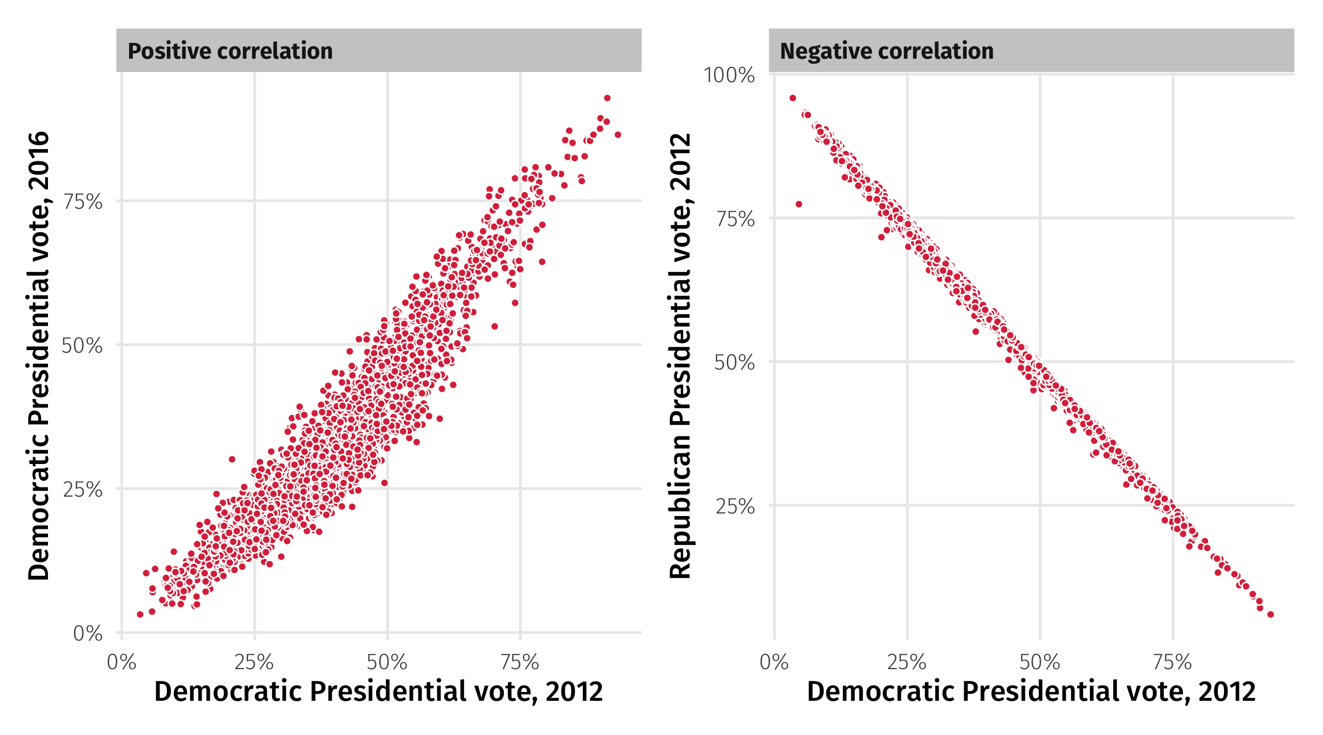
Correlation: direction
➕: When two variables move “in the same direction”
➖: When two variables move “in opposite directions”
Interpreting the coefficient
| Correlation coefficient | Rough meaning |
|---|---|
| +/- 0.1 - 0.3 | Modest |
| +/- 0.3 - 0.5 | Moderate |
| +/- 0.5 - 0.8 | Strong |
| +/- 0.8 - 0.9 | Very strong |

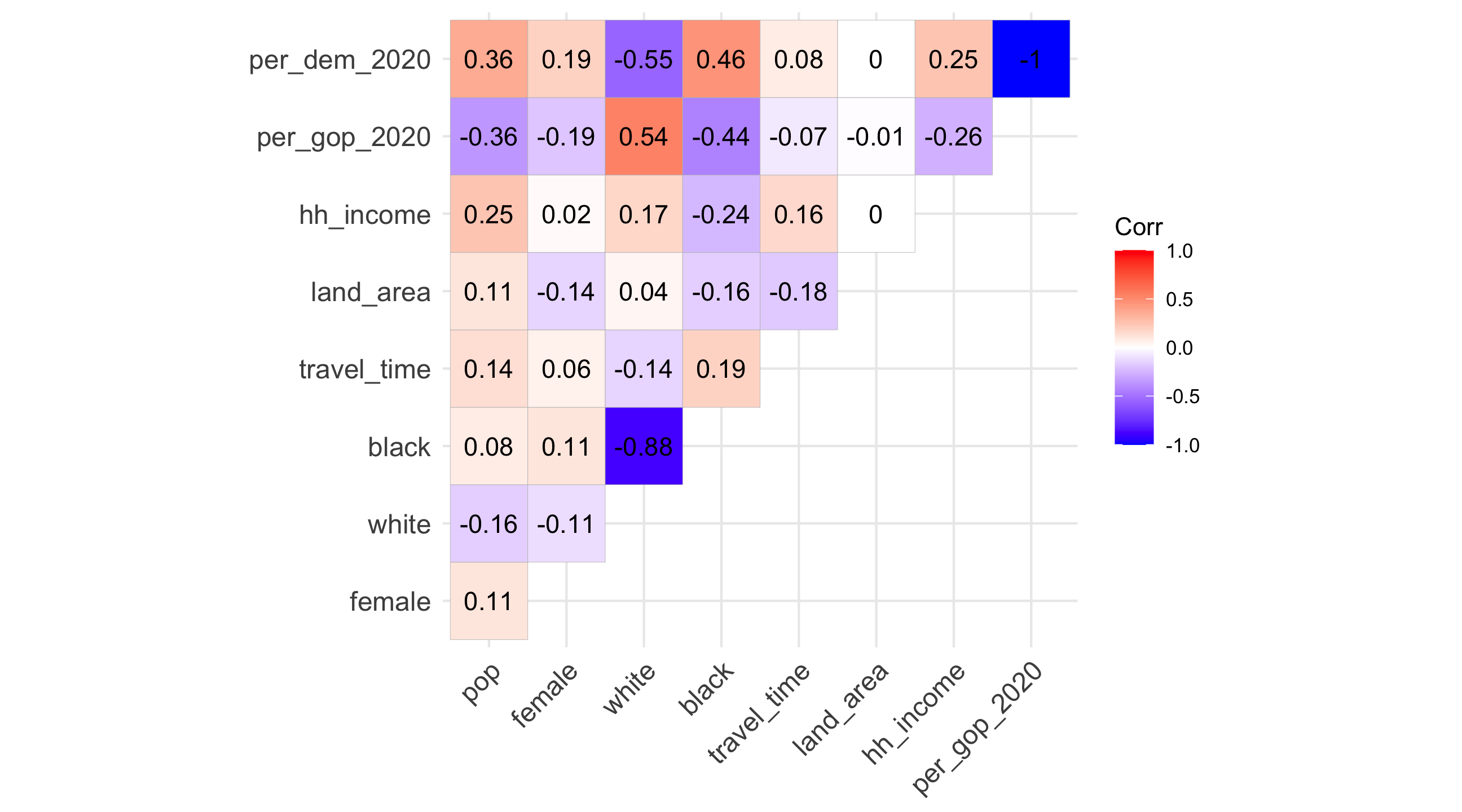
🚨 Our turn: correlations 🚨
What do these pair-wise correlations from elections tell us?
Models
Models are everywhere in social science (and industry)
Beneath what ads you see, movie recs, election forecasts, social science research \(\rightarrow\) a model
In the social sciences, we use models to describe how an outcome changes in response to a treatment

The moving parts
The things we want to study in the social sciences are complex
Why do people vote? We can think of lots of factors that go into this decision
Voted = Age + Interest in politics + Free time + Social networks + . . .
Models break up (decompose) the variance in an outcome into a set of explanatory variables

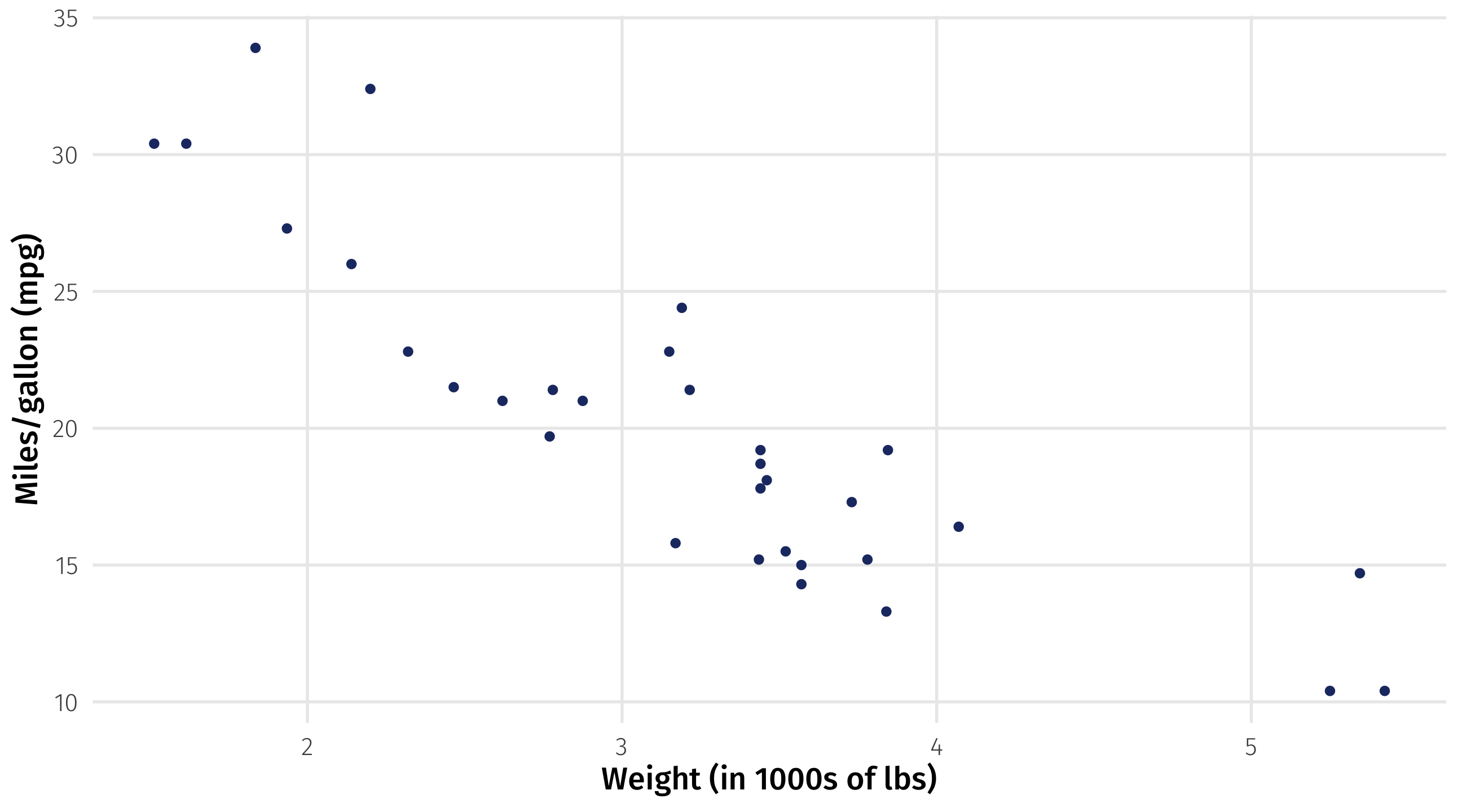
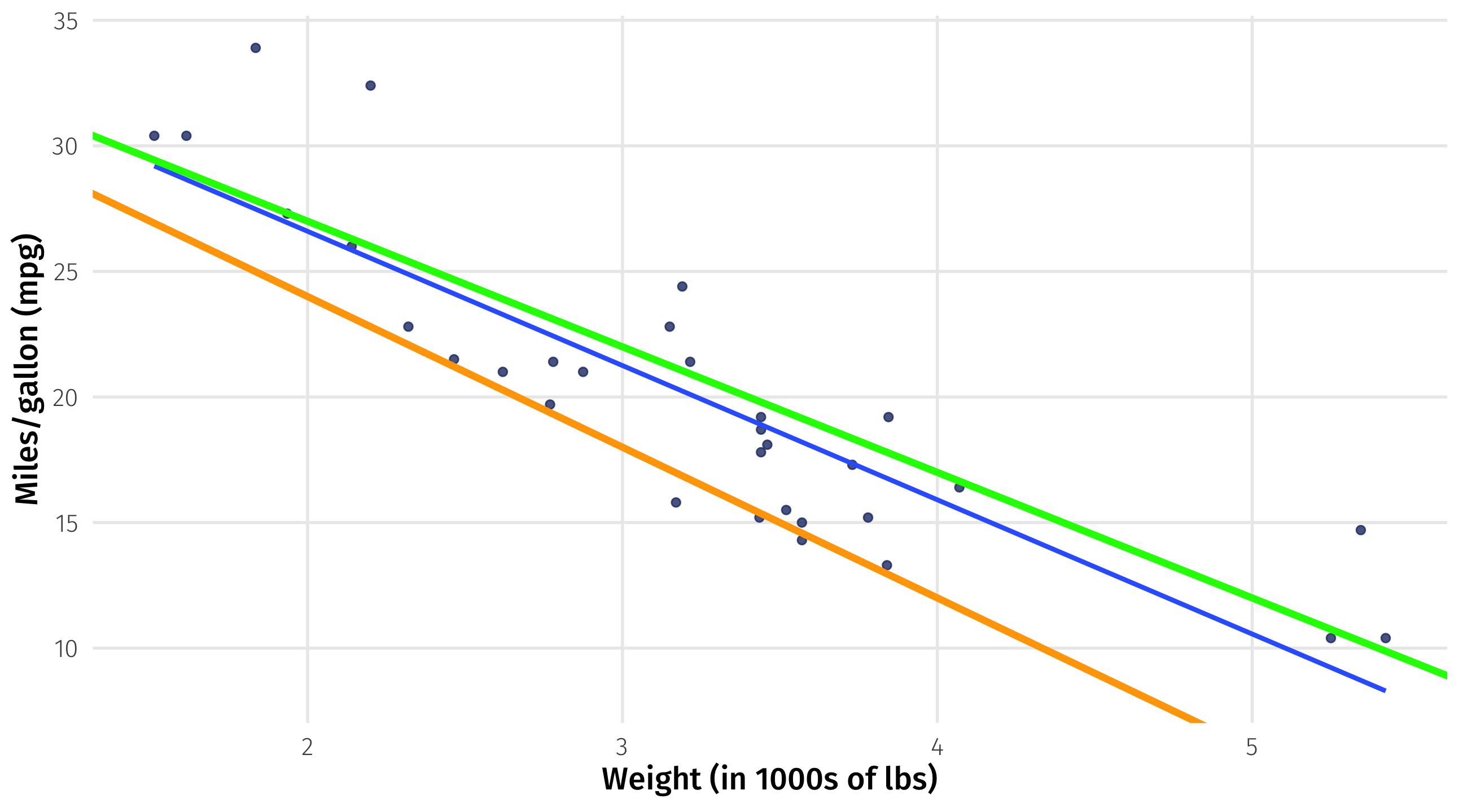
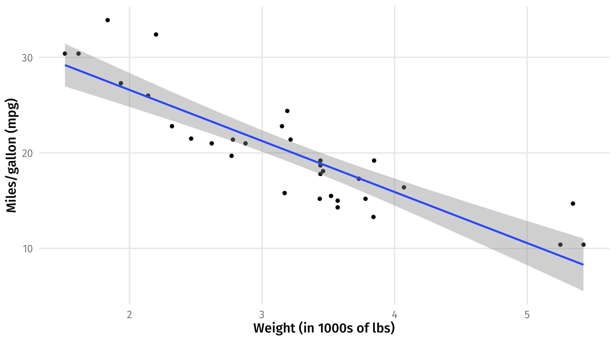
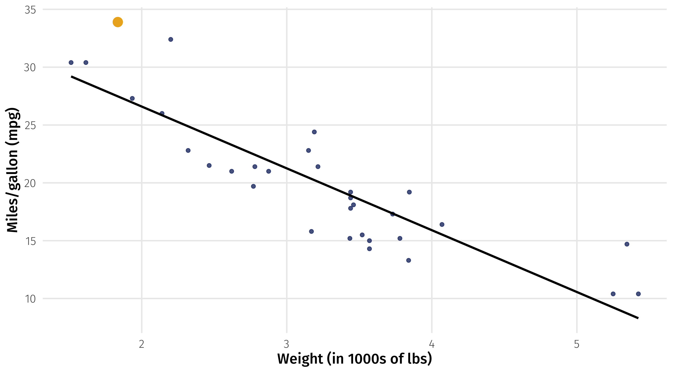
Modeling weight and fuel efficiency
Very strong, negative correlation (r = -.9)
Why a model?
Graph + correlation just gives us direction and strength of relationship
What if we wanted to know what fuel efficiency to expect if a car weighs 3 tons, or 6.2?
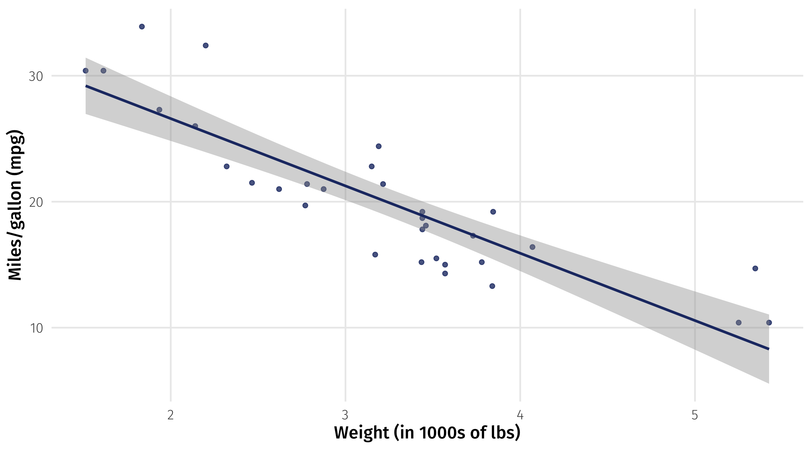
Lines as models
There’s many ways to model relationships between variables
A simple model is a line that “fits” the data “well”
The line of best fit describes how fuel efficiency changes as weight changes

Strength of relationship
The slope of the line quantifies the strength of the relationship
Slope: -5.3 \(\rightarrow\) for every ton of weight you add to a car, you lose 5 miles per gallon
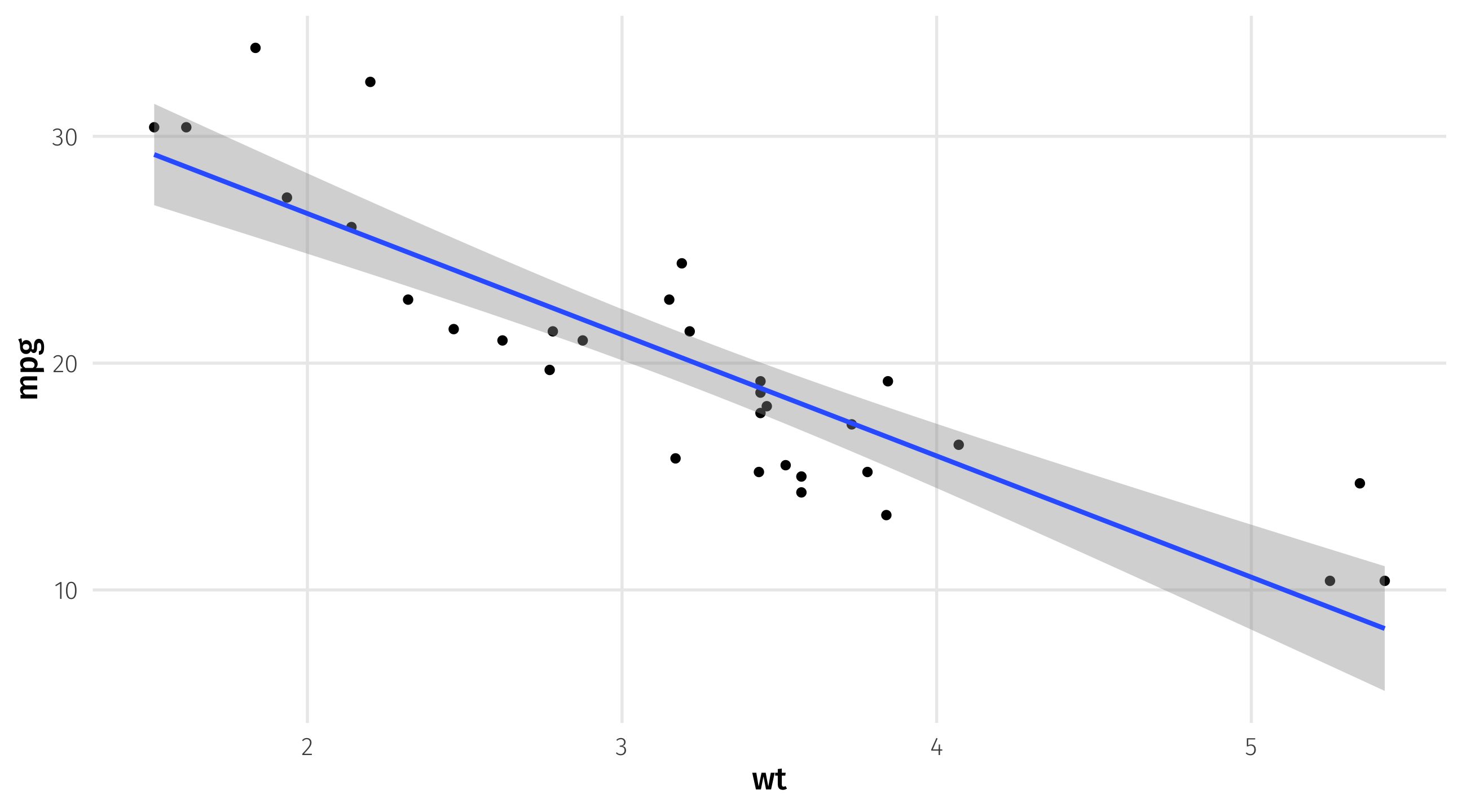
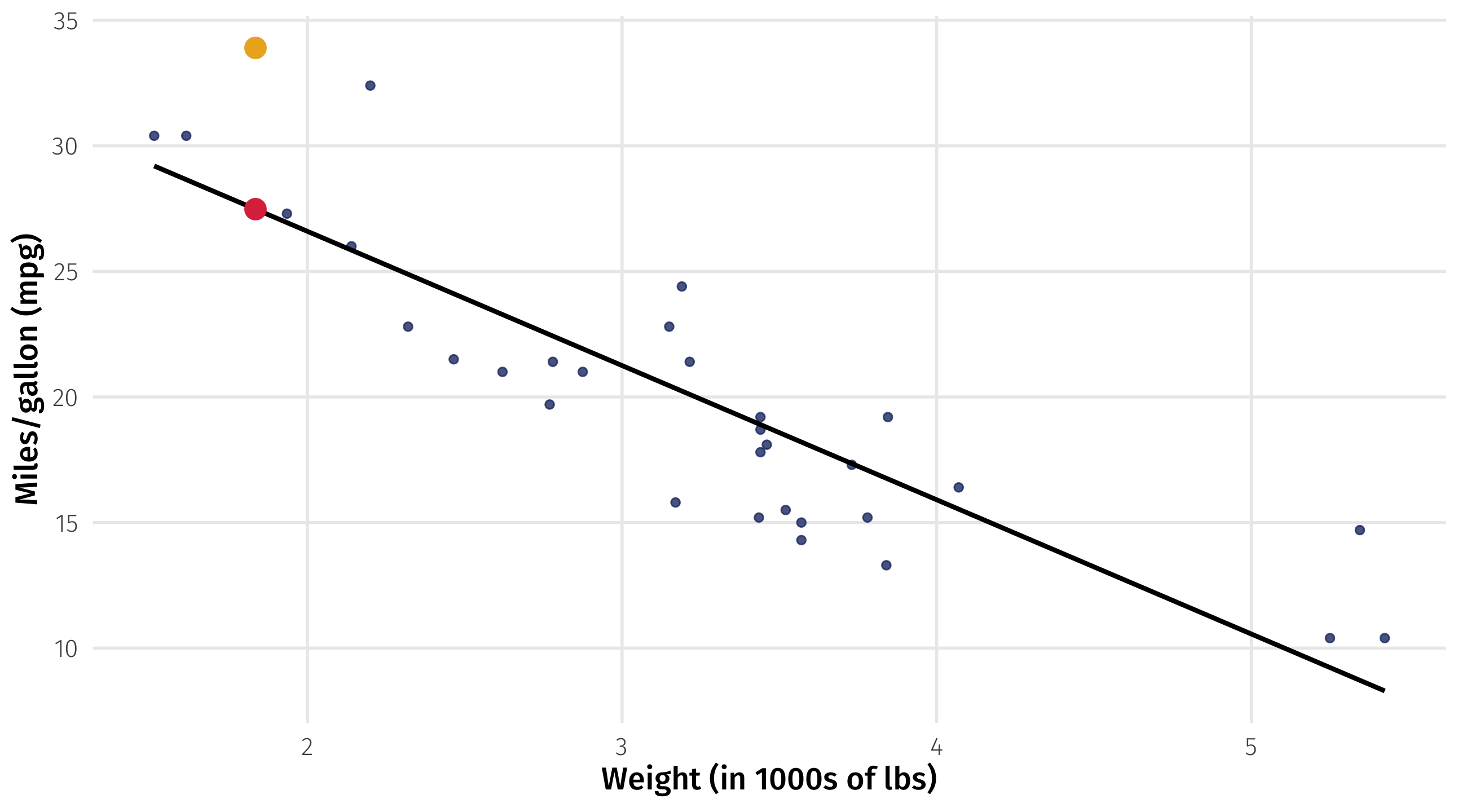
Guessing where there’s no data
Line also gives us “best guess” for the fuel efficiency of a car with a given weight
even where we have no data
best guess for 4.5 ton car \(\rightarrow\) 13 mpg

Drawing lines in R
We can add a trend-line to a graph using geom_smooth(method = "lm")
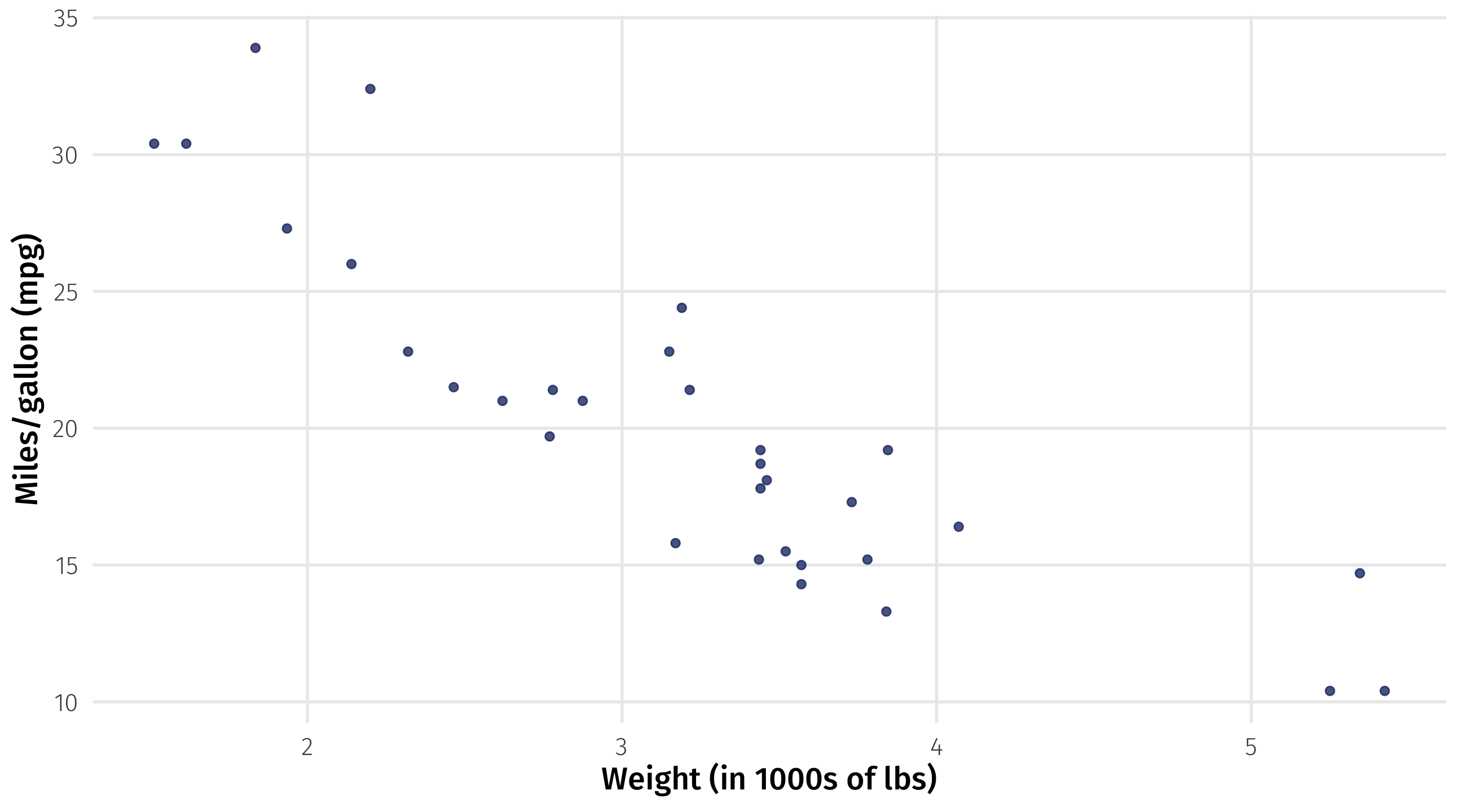
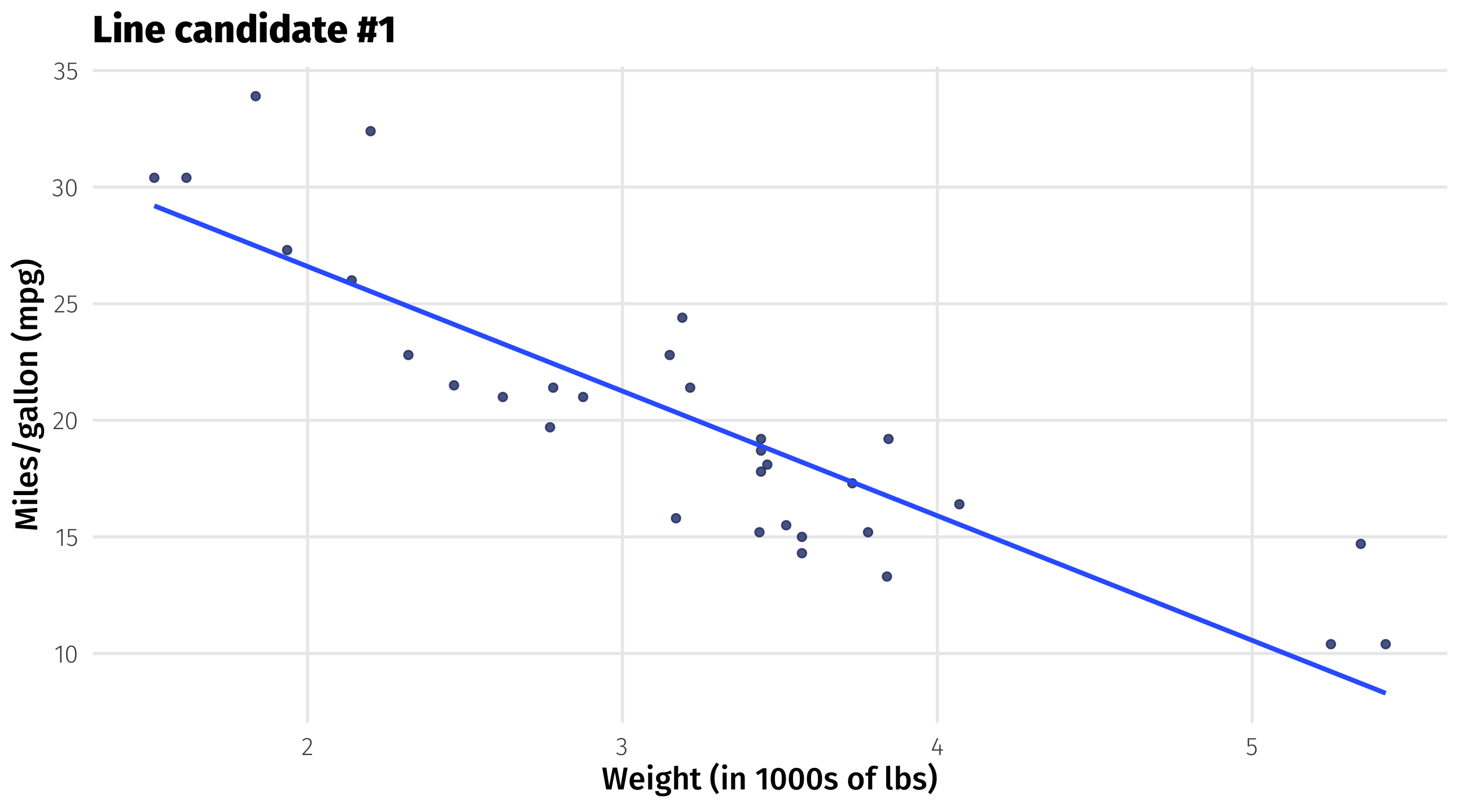
Some lines
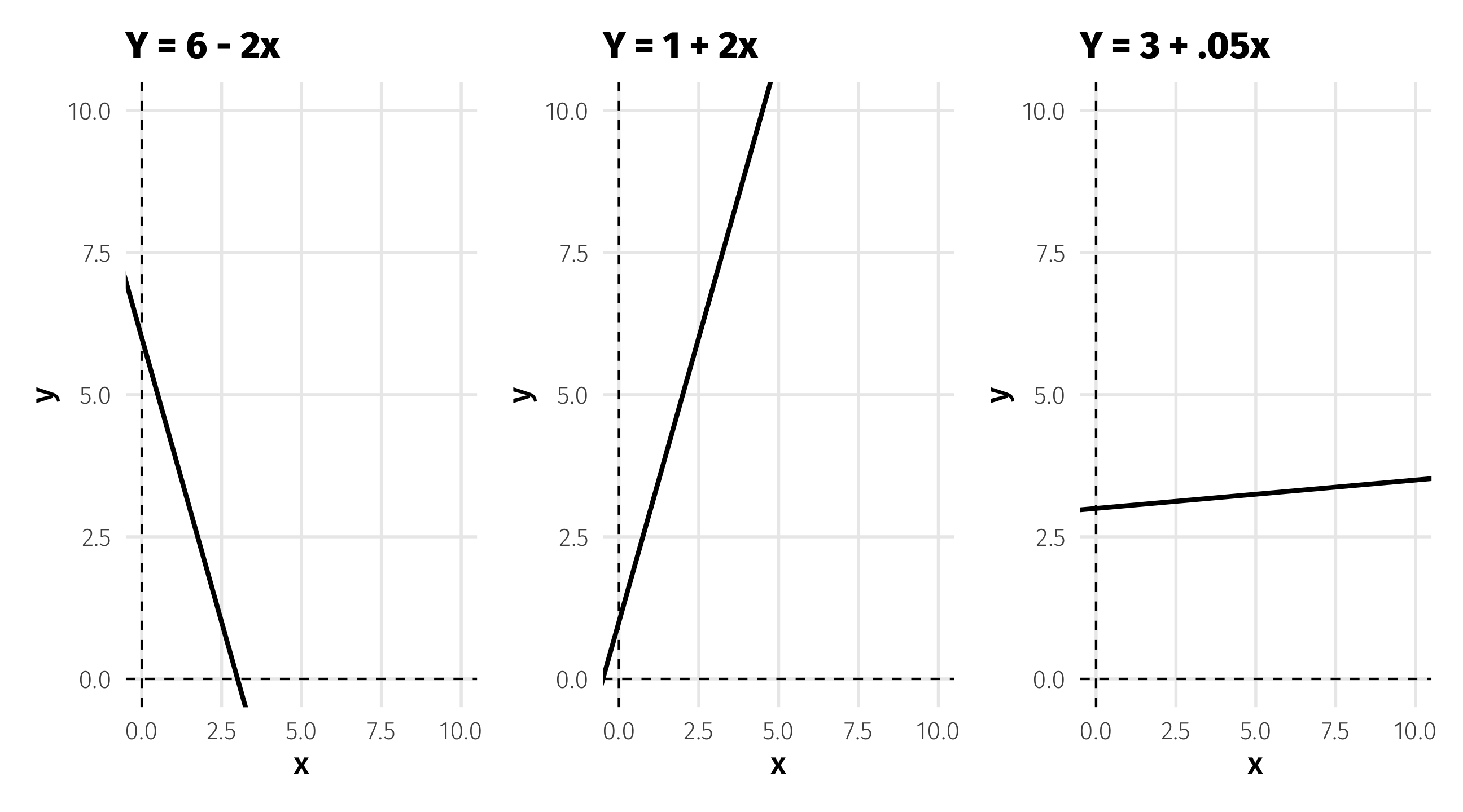
Which line to draw?
We could draw many lines through this data; which is “best”?
Drawing the line
We need to find the intercept (\(\beta_0\)) and slope (\(\beta_1\)) that will “fit” the data “well”
\(mpg_{i} = \beta_0 + \beta_1 \times weight_{i}\)
What does it mean to “fit well”?
- Models use a rule for defining what it means to fit the data “well”
- This rule is called a loss function
- Different models use different loss functions
- We’ll look at the most popular modeling approach:
- ordinary least squares (OLS)
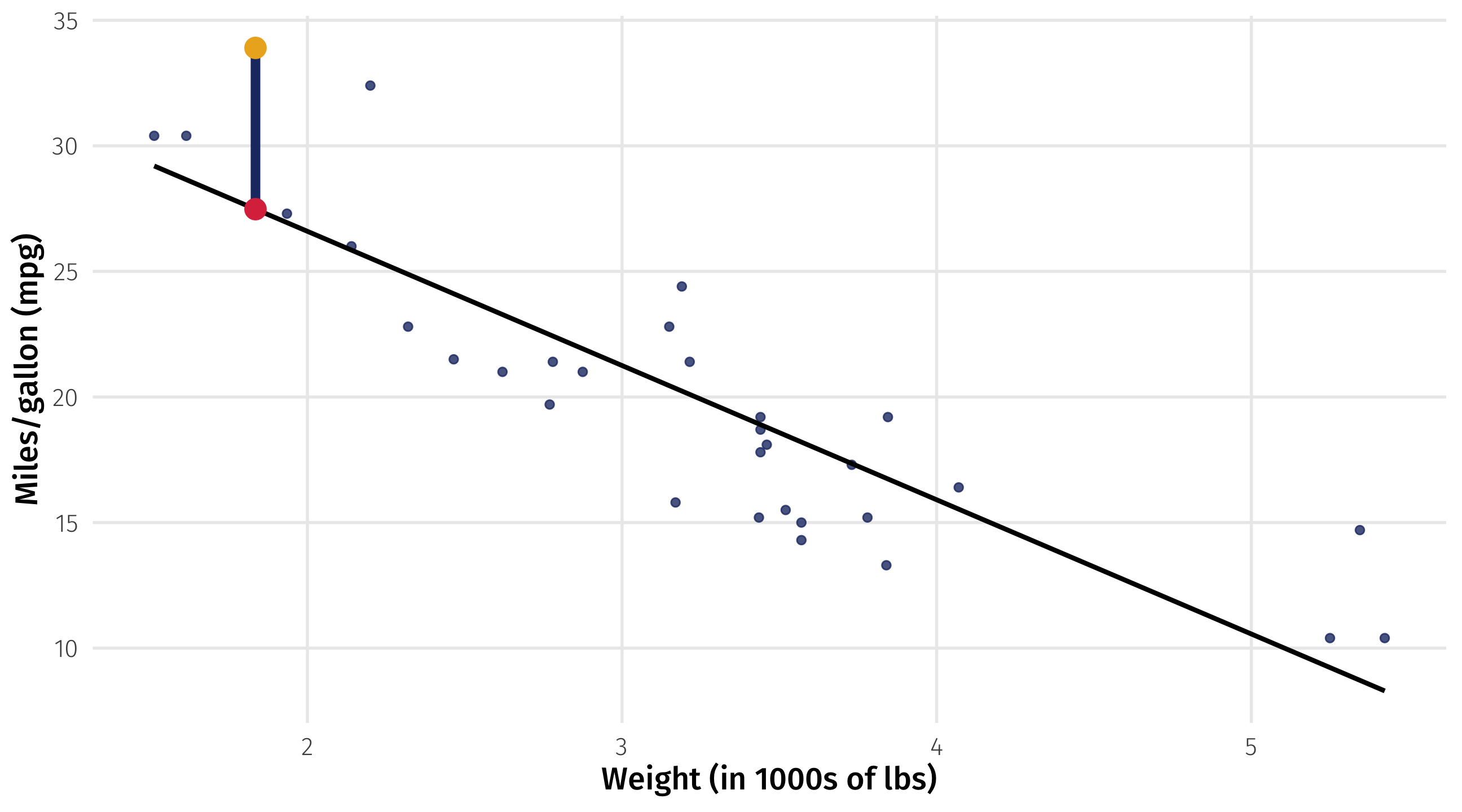
Distance between each point and the line
\(Y_i\) = actual MPG for the Toyota Corolla
Distance between each point and the line
\(\widehat{Y_i}\) = our model’s predicted MPG (\(\beta_0\) + \(\beta_1 \times weight\)) for the Corolla
Distance between each point and the line
\(Y_i - \widehat{Y_i}\) = the distance between the data point and the line
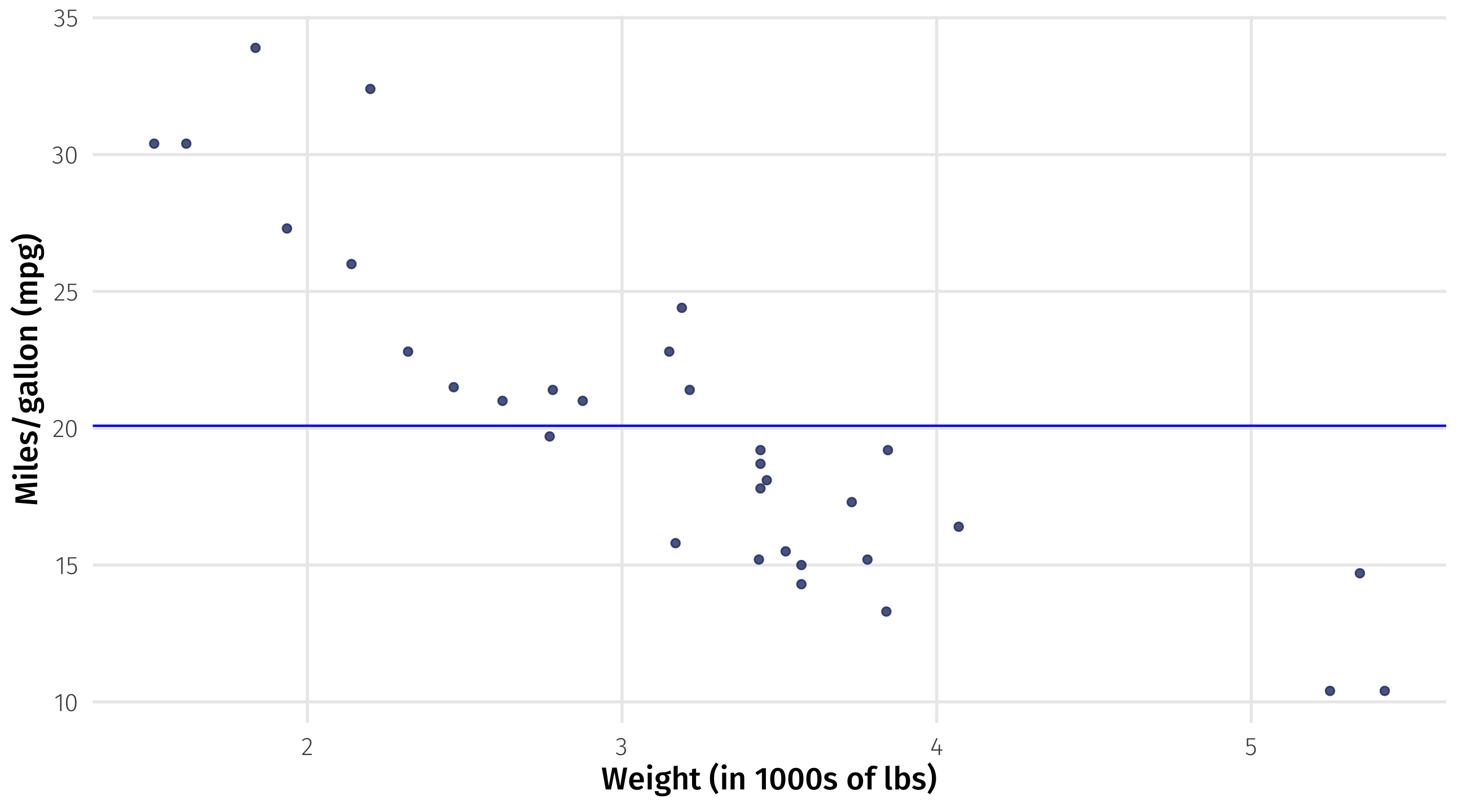
Strawman comparison
Which line fits the data better? (Duh)
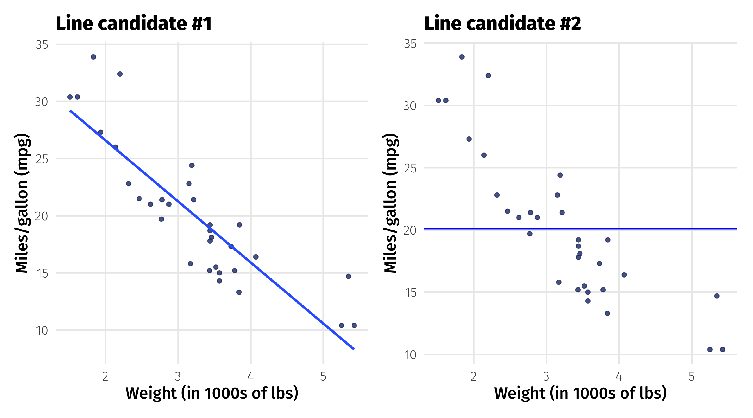
First candidate: fit the line
Rough guess: what is \(\beta_0\) and \(\beta_1\) here?
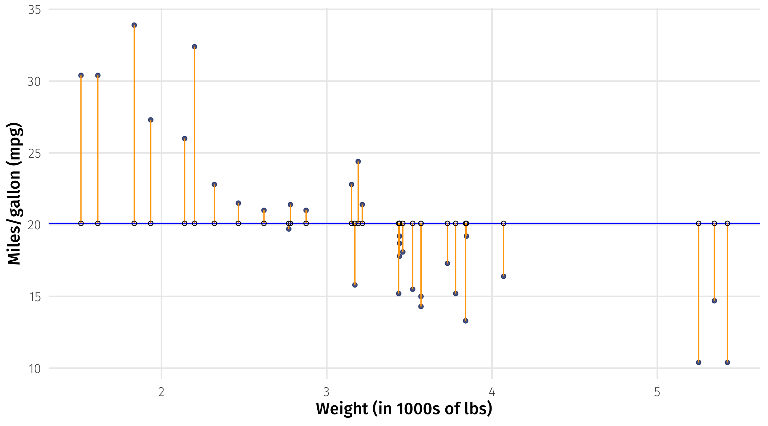
First candidate: the residuals
How far is each point from the line? This is \((Y_i - \widehat{Y_i})\)
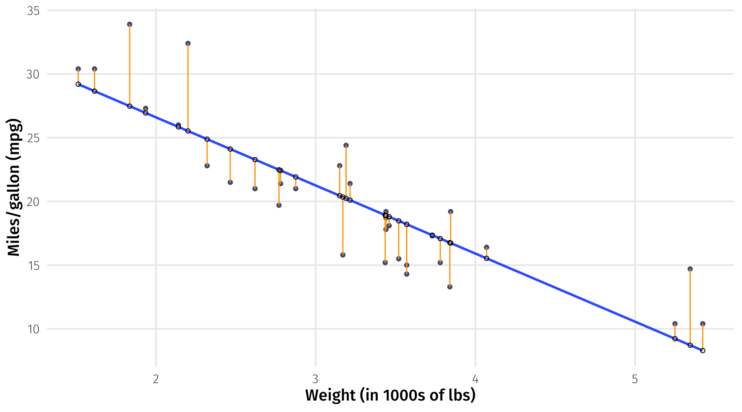
Also known as the residual \(\approx\) how wrong the line is about each point
Second candidate: fit the line
Rough guess: what is \(\beta_0\) and \(\beta_1\) here?
Second candidate: the residuals
So who are the winning Betas?
\(Y = \beta_0 + \beta1x_1\)
\(mpg = \beta_0 + \beta_1 \times weight\)
\(mpg = 37 + -5 \times weight\)

Modeling in a nutshell
You want to see how some outcome responds to some treatment
Fit a line (or something else) to the variables
Extract the underlying model
Use the model to make inferences