Relationships II

POL51

Juan F. Tellez

University of California, Davis

December 5, 2023

Plan for today

Comparing across groups

Dummy variables

Summarizing categories

Comparing across groups

The feeling thermometer

We can use summarise() to measure average support for specific groups:

therm %>% 
  summarise(avg_police = mean(ft_police, na.rm = TRUE)) 

# A tibble: 1 × 1
  avg_police
       <dbl>
1       75.7

Feeling thermometer

We can compare where support is highest and lowest:

therm %>% 
  summarise(avg_police = mean(ft_police, na.rm = TRUE), 
            avg_muslim = mean(ft_muslim, na.rm = TRUE), 
            avg_white = mean(ft_white, na.rm = TRUE), 
            avg_immig = mean(ft_immig, na.rm = TRUE), 
            avg_fem = mean(ft_fem, na.rm = TRUE), 
            avg_black = mean(ft_black, na.rm = TRUE)) 

# A tibble: 1 × 6
  avg_police avg_muslim avg_white avg_immig avg_fem avg_black
       <dbl>      <dbl>     <dbl>     <dbl>   <dbl>     <dbl>
1       75.7       50.0      76.1      61.9    52.1      71.3

patterns

Breaking down support

We can look for patterns by using group_by() to separate average support by respondent characteristics:

therm %>% 
  group_by(party_id) %>% 
  summarise(avg_police = mean(ft_police, na.rm = TRUE), 
            avg_muslim = mean(ft_muslim, na.rm = TRUE), 
            avg_white = mean(ft_white, na.rm = TRUE), 
            avg_immig = mean(ft_immig, na.rm = TRUE), 
            avg_fem = mean(ft_fem, na.rm = TRUE), 
            avg_black = mean(ft_black, na.rm = TRUE))

# A tibble: 5 × 7
  party_id    avg_police avg_muslim avg_white avg_immig avg_fem avg_black
  <fct>            <dbl>      <dbl>     <dbl>     <dbl>   <dbl>     <dbl>
1 Democrat          67.8       64.6      74.1      71.7    73.9      78.3
2 Republican        87.6       33.3      81.7      50.2    30.3      65.6
3 Independent       74.2       49.0      74.1      61.5    48.3      69.1
4 Other             72.7       45.1      71.1      65.4    40.7      70.2
5 Not sure          70.1       47.1      70.8      56.9    54.0      66.7

take code and iteratively change it

Breaking down support

We can use filter() to focus our comparison on fewer categories:

therm_by_party = therm %>% 
  filter(party_id %in% c("Democrat", "Republican")) %>% 
  group_by(party_id) %>% 
  summarise(avg_police = mean(ft_police, na.rm = TRUE), 
            avg_muslim = mean(ft_muslim, na.rm = TRUE), 
            avg_white = mean(ft_white, na.rm = TRUE), 
            avg_immig = mean(ft_immig, na.rm = TRUE), 
            avg_fem = mean(ft_fem, na.rm = TRUE), 
            avg_black = mean(ft_black, na.rm = TRUE))
therm_by_party

# A tibble: 2 × 7
  party_id   avg_police avg_muslim avg_white avg_immig avg_fem avg_black
  <fct>           <dbl>      <dbl>     <dbl>     <dbl>   <dbl>     <dbl>
1 Democrat         67.8       64.6      74.1      71.7    73.9      78.3
2 Republican       87.6       33.3      81.7      50.2    30.3      65.6

Where are the biggest partisan gaps? What’s going on with immigrants? Is this really an apples-to-apples comparison?

The immigration gap

What explains this gap? How much is it about each party’s ideology and how much is about who is in each party?

Immigrants in the USA are more likely to identify as Democrat

How much of the difference we are observing across parties solely about parties and how much is it about demographic differences?

It might be, for instance, that the attitudes of non-migrants don’t differ much across parties

that is, the big gap we see is all because immigrants are both more likely to be Democrats and have stronger views of own community

Making sense of the immigration gap

We want an apples to apples comparison: White Dems vs. White Reps, Asian Dems vs. Asian Reps, and so on

We can “test” this concern by breaking the data down further, by race:

therm %>% 
  filter(party_id %in% c("Democrat", "Republican")) %>%
  group_by(party_id, race) %>%
  summarise(avg_imm = mean(ft_immig, na.rm = TRUE))

# A tibble: 14 × 3
# Groups:   party_id [2]
   party_id   race            avg_imm
   <fct>      <fct>             <dbl>
 1 Democrat   White              71.2
 2 Democrat   Black              71.1
 3 Democrat   Hispanic           76.2
 4 Democrat   Asian              75.5
 5 Democrat   Native American    62.9
 6 Democrat   Mixed              74.6
 7 Democrat   Other              84.1
 8 Republican White              49.8
 9 Republican Black              54.6
10 Republican Hispanic           58.0
11 Republican Asian              54.7
12 Republican Native American    47.4
13 Republican Mixed              51.4
14 Republican Other              42.3

Making sense of the immigration gap

We can filter to focus on fewer races:

therm %>% 
  filter(party_id %in% c("Democrat", "Republican")) %>%
  filter(race %in% c("White", "Black", "Hispanic", "Asian")) |> 
  group_by(party_id, race) %>%
  summarise(avg_imm = mean(ft_immig, na.rm = TRUE))

# A tibble: 8 × 3
# Groups:   party_id [2]
  party_id   race     avg_imm
  <fct>      <fct>      <dbl>
1 Democrat   White       71.2
2 Democrat   Black       71.1
3 Democrat   Hispanic    76.2
4 Democrat   Asian       75.5
5 Republican White       49.8
6 Republican Black       54.6
7 Republican Hispanic    58.0
8 Republican Asian       54.7

Visualizing the pattern

We can create a new object to make a nice plot:

therm_party_immig = therm %>% 
  filter(party_id %in% c("Democrat", "Republican")) %>%
  filter(race %in% c("White", "Black", "Hispanic", "Asian")) |> 
  group_by(party_id, race) %>%
  summarise(avg_imm = mean(ft_immig, na.rm = TRUE))

The immigration attitudes gap

comparing apples to apples, the gap persists

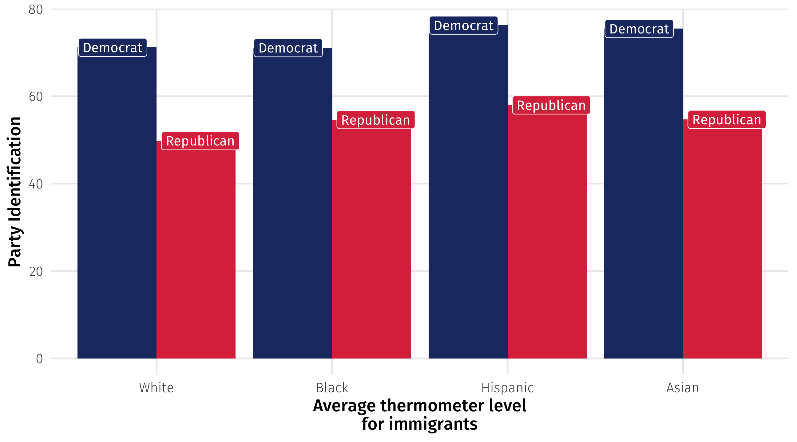
Big picture

The immigration gap persists (though smaller), even comparing non-immigrants against non-immigrants and immigrants against immigrants

This analysis is a way of accounting for differences in groups (Democrats versus Republicans); it’s closer to an “apples to apples” comparison

Big differences across groups should raise eyebrows; what’s going on here?

We can break the data down further to see what’s going on beneath the surface

Non-differences can be surprsing too

therm %>% 
  summarise(avg_dems = mean(ft_dem, na.rm = TRUE), 
            avg_reps = mean(ft_rep, na.rm = TRUE))

# A tibble: 1 × 2
  avg_dems avg_reps
     <dbl>    <dbl>
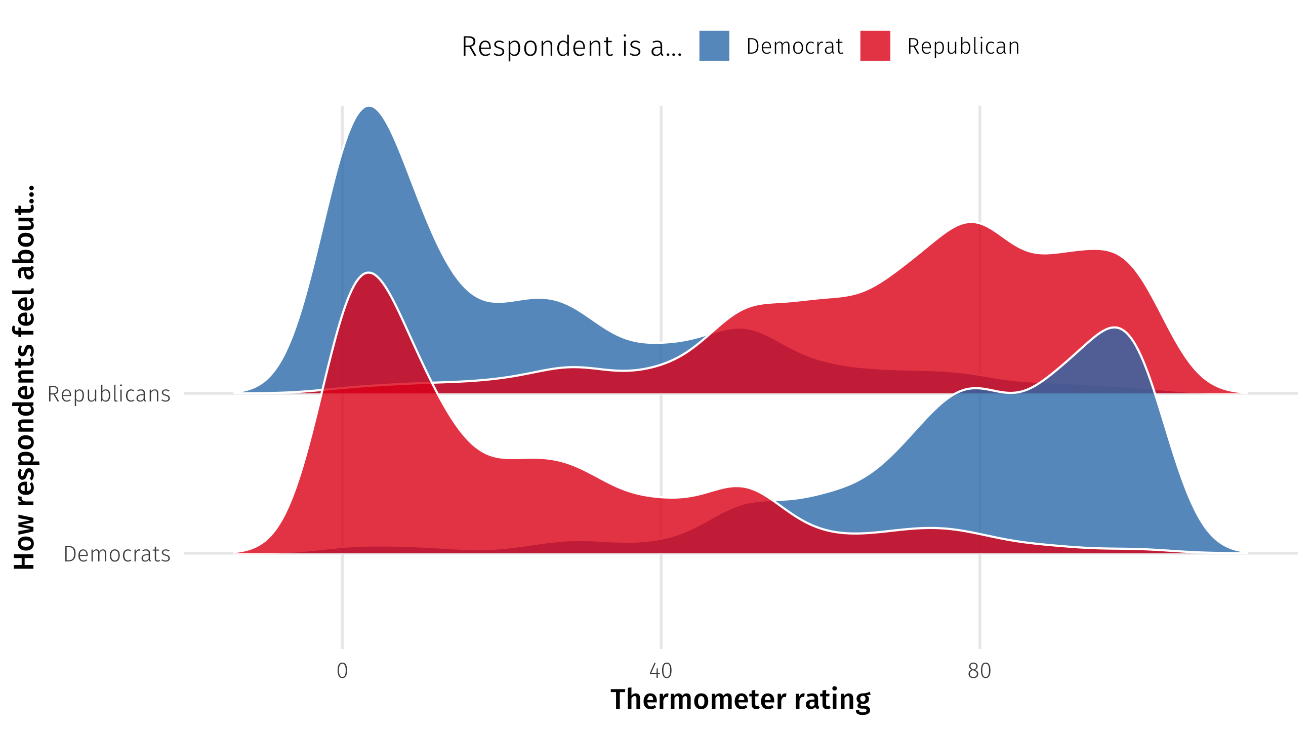
1     49.4     43.3

Pretty neutral feelings; mass polarization is dead!

Oh…

Breaking down data says something different

therm %>% 
  group_by(party_id) %>% #<<
  summarise(dems = mean(ft_dem, na.rm = TRUE), 
            reps = mean(ft_rep, na.rm = TRUE))

# A tibble: 5 × 3
  party_id     dems  reps
  <fct>       <dbl> <dbl>
1 Democrat     79.9  22.1
2 Republican   21.5  72.4
3 Independent  41.2  39.6
4 Other        31.9  38.7
5 Not sure     43.2  42.3

Negative polarization

Dummy variables

Dummy variables

Often, categorical variables are coded 0/1 to represent “yes/no” or “presence/absence”

sample from leaders dataset

country	leader	mil_service	combat
BOT	Khama	0	0
RUS	Nicholas II	1	0
MEX	Salinas	0	0
MAA	Sidi Ahmed Taya	1	1
CHL	Frei Montalva	0	0
LEB	Chamoun	0	0
GRC	Tsokhatzopulos	0	0
COL	Nel Ospina	1	1
OMA	Taimur ibn Faysal	0	0
BNG	Hasina Wazed	NA	NA

Dummy proportions

Dummy variables are useful for lots of reasons

One is that when you take the average of a dummy variable you get a proportion

Coffee today? 1, 0, 0, 0, 1

Average of coffee = \(\frac{1 + 0 + 0 + 0 + 1}{5} = .40\)

We can think about that proportion as a probability or likelihood

What is the probability a random student in class has had coffee? 2/5 = 40%

Dummy variables

When you take the average of a dummy variable you get a proportion:

leader %>% 
  summarise(combat = mean(combat, na.rm = TRUE)) 

# A tibble: 1 × 1
  combat
   <dbl>
1  0.246

Approximately 24% of world leaders have combat experience, or

there’s a 24% chance a randomly selected leader has combat experience

Dummy variables

Like with anything else, we can take averages by groups

For example, combat experience by country

leader %>% 
  group_by(country) %>%
  summarise(combat = mean(combat, na.rm = TRUE)) |> 
  arrange(desc(combat))

# A tibble: 189 × 2
   country combat
   <chr>    <dbl>
 1 AUH      0.958
 2 TAJ      0.857
 3 BFO      0.817
 4 TOG      0.816
 5 NIG      0.780
 6 PRK      0.723
 7 BEN      0.683
 8 EQG      0.673
 9 NIR      0.667
10 CON      0.667
# ℹ 179 more rows

Note that arrange(desc(variable)) arranges the dataset in descending order

Dummy variables

We can store as an object, to make a plot:

combat_country = leader %>% 
  group_by(country) %>%
  # proportion who've seen combat
  summarise(combat = mean(combat, na.rm = TRUE)) |> 
  # subset to just the top 10 in terms of combat experience
  slice_max(order_by = combat, n = 10)

ggplot(combat_country, aes(y = reorder(country, combat),
                           x = combat)) + 
  geom_col()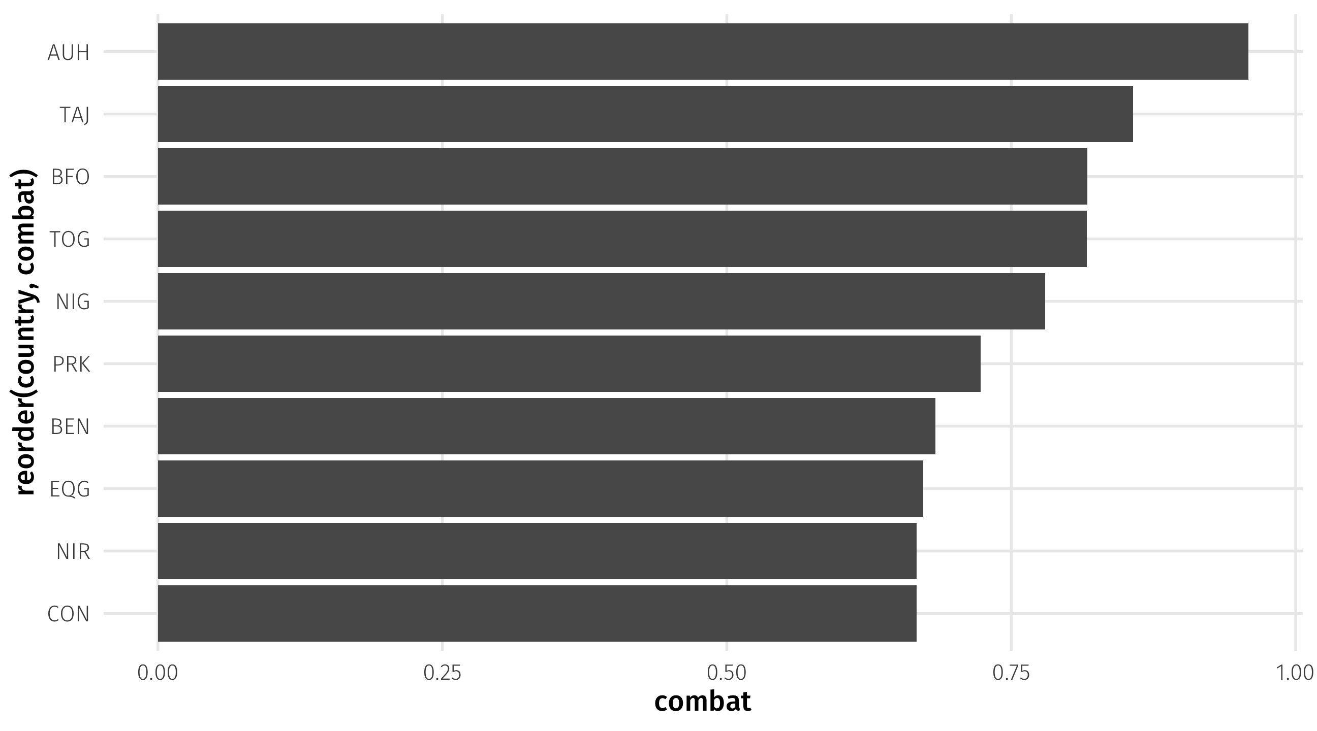

🚨 Your turn: 🎨 Bob Ross 🎨 🚨

episode	season	episode_num	title	apple_frame	aurora_borealis	barn	beach	boat	bridge	building	bushes	cabin	cactus	circle_frame	cirrus	cliff	clouds	conifer	cumulus	deciduous	diane_andre	dock	double_oval_frame	farm	fence	fire	florida_frame	flowers	fog	framed	grass	guest	half_circle_frame	half_oval_frame	hills	lake	lakes	lighthouse	mill	moon	mountain	mountains	night	ocean	oval_frame	palm_trees	path	person	portrait	rectangle_3d_frame	rectangular_frame	river	rocks	seashell_frame	snow	snowy_mountain	split_frame	steve_ross	structure	sun	tomb_frame	tree	trees	triple_frame	waterfall	waves	windmill	window_frame	winter	wood_framed
S01E01	1	1	A WALK IN THE WOODS	0	0	0	0	0	0	0	1	0	0	0	0	0	0	0	0	1	0	0	0	0	0	0	0	0	0	0	1	0	0	0	0	0	0	0	0	0	0	0	0	0	0	0	0	0	0	0	0	1	0	0	0	0	0	0	0	0	0	1	1	0	0	0	0	0	0	0
S01E02	1	2	MT. MCKINLEY	0	0	0	0	0	0	0	0	1	0	0	0	0	1	1	0	0	0	0	0	0	0	0	0	0	0	0	0	0	0	0	0	0	0	0	0	0	1	0	0	0	0	0	0	0	0	0	0	0	0	0	1	1	0	0	0	0	0	1	1	0	0	0	0	0	1	0
S01E03	1	3	EBONY SUNSET	0	0	0	0	0	0	0	0	1	0	0	0	0	0	1	0	0	0	0	0	0	1	0	0	0	0	0	0	0	0	0	0	0	0	0	0	0	1	1	0	0	0	0	0	0	0	0	0	0	0	0	0	0	0	0	1	1	0	1	1	0	0	0	0	0	1	0
S01E04	1	4	WINTER MIST	0	0	0	0	0	0	0	1	0	0	0	0	0	1	1	0	0	0	0	0	0	0	0	0	0	0	0	0	0	0	0	0	1	0	0	0	0	1	0	0	0	0	0	0	0	0	0	0	0	0	0	0	1	0	0	0	0	0	1	1	0	0	0	0	0	0	0
S01E05	1	5	QUIET STREAM	0	0	0	0	0	0	0	0	0	0	0	0	0	0	0	0	1	0	0	0	0	0	0	0	0	0	0	0	0	0	0	0	0	0	0	0	0	0	0	0	0	0	0	0	0	0	0	0	1	1	0	0	0	0	0	0	0	0	1	1	0	0	0	0	0	0	0
S01E06	1	6	WINTER MOON	0	0	0	0	0	0	0	0	1	0	0	0	0	0	1	0	0	0	0	0	0	0	0	0	0	0	0	0	0	0	0	0	1	0	0	0	1	1	1	1	0	0	0	0	0	0	0	0	0	0	0	1	1	0	0	1	0	0	1	1	0	0	0	0	0	1	0

🚨 Your turn: 🎨 Bob Ross 🎨 🚨

Using the bob_ross data from fivethirtyeight package

1. How likely was Bob Ross to include a happy little tree in one of his paintings?

2. How has the frequency with which Bob Ross included clouds in his paintings changed across the show’s seasons? Make a time series to illustrate.

3. If there is a mountain in a Bob Ross painting, how likely is it that mountain is snowy (snowy_mountain)?

4. How much more likely was Steve Ross (steve) to paint a lake (lake) than his dad?

10:00

Analyzing categorical data

Analyzing categorical data

Some variables have values that are categories (race, sex, etc.)

Can’t take the mean of a category!

But we can look at the proportions of observations in each category, and look for patterns there

Pokemon types

How many Pokemon are there of each type? What are the most and least common types?

name	type1
Vaporeon	water
Clawitzer	water
Regirock	rock
Torterra	grass
Salandit	poison
Mareep	electric
Blaziken	fire

Counting categories

We can use a new function tally(), in combination with group_by(), to count how many observations are in each category:

pokemon

# A tibble: 801 × 14
   name       type1 type2  height_m weight_kg capture_rate    hp attack defense
   <chr>      <chr> <chr>     <dbl>     <dbl>        <dbl> <dbl>  <dbl>   <dbl>
 1 Bulbasaur  grass poison      0.7       6.9           45    45     49      49
 2 Ivysaur    grass poison      1        13             45    60     62      63
 3 Venusaur   grass poison      2       100             45    80    100     123
 4 Charmander fire  <NA>        0.6       8.5           45    39     52      43
 5 Charmeleon fire  <NA>        1.1      19             45    58     64      58
 6 Charizard  fire  flying      1.7      90.5           45    78    104      78
 7 Squirtle   water <NA>        0.5       9             45    44     48      65
 8 Wartortle  water <NA>        1        22.5           45    59     63      80
 9 Blastoise  water <NA>        1.6      85.5           45    79    103     120
10 Caterpie   bug   <NA>        0.3       2.9          255    45     30      35
# ℹ 791 more rows
# ℹ 5 more variables: sp_attack <dbl>, sp_defense <dbl>, speed <dbl>,
#   generation <dbl>, is_legendary <dbl>

Counting categories

We can use a new function tally(), in combination with group_by(), to count how many observations are in each category:

pokemon %>% 
  group_by(type1) 

# A tibble: 801 × 14
# Groups:   type1 [18]
   name       type1 type2  height_m weight_kg capture_rate    hp attack defense
   <chr>      <chr> <chr>     <dbl>     <dbl>        <dbl> <dbl>  <dbl>   <dbl>
 1 Bulbasaur  grass poison      0.7       6.9           45    45     49      49
 2 Ivysaur    grass poison      1        13             45    60     62      63
 3 Venusaur   grass poison      2       100             45    80    100     123
 4 Charmander fire  <NA>        0.6       8.5           45    39     52      43
 5 Charmeleon fire  <NA>        1.1      19             45    58     64      58
 6 Charizard  fire  flying      1.7      90.5           45    78    104      78
 7 Squirtle   water <NA>        0.5       9             45    44     48      65
 8 Wartortle  water <NA>        1        22.5           45    59     63      80
 9 Blastoise  water <NA>        1.6      85.5           45    79    103     120
10 Caterpie   bug   <NA>        0.3       2.9          255    45     30      35
# ℹ 791 more rows
# ℹ 5 more variables: sp_attack <dbl>, sp_defense <dbl>, speed <dbl>,
#   generation <dbl>, is_legendary <dbl>

Counting categories

We can use a new function tally(), in combination with group_by(), to count how many observations are in each category:

pokemon %>% 
  group_by(type1) %>% 
  tally() 

# A tibble: 18 × 2
   type1        n
   <chr>    <int>
 1 bug         72
 2 dark        29
 3 dragon      27
 4 electric    39
 5 fairy       18
 6 fighting    28
 7 fire        52
 8 flying       3
 9 ghost       27
10 grass       78
11 ground      32
12 ice         23
13 normal     105
14 poison      32
15 psychic     53
16 rock        45
17 steel       24
18 water      114

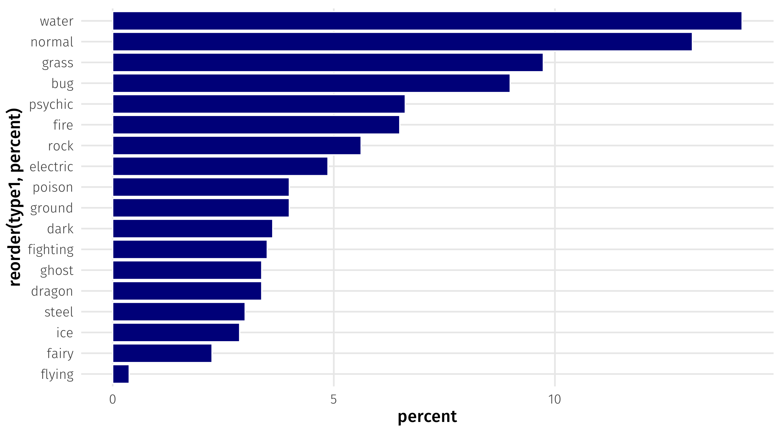
From counts to percents

We can can then use mutate() to calculate the percent in each group:

pokemon %>% 
  group_by(type1) %>% 
  tally() %>% 
  mutate(percent = n / sum(n) * 100) 

# A tibble: 18 × 3
   type1        n percent
   <chr>    <int>   <dbl>
 1 bug         72   8.99 
 2 dark        29   3.62 
 3 dragon      27   3.37 
 4 electric    39   4.87 
 5 fairy       18   2.25 
 6 fighting    28   3.50 
 7 fire        52   6.49 
 8 flying       3   0.375
 9 ghost       27   3.37 
10 grass       78   9.74 
11 ground      32   4.00 
12 ice         23   2.87 
13 normal     105  13.1  
14 poison      32   4.00 
15 psychic     53   6.62 
16 rock        45   5.62 
17 steel       24   3.00 
18 water      114  14.2  

stop to show the n/sum(n)

group_by + tally()

We can then store as object for plotting:

type_pct = pokemon %>% 
  group_by(type1) %>% 
  tally() %>% 
  mutate(percent = n/sum(n) * 100)

group_by + tally()

We can then store as object for plotting:

ggplot(type_pct, aes(y = reorder(type1, percent), 
                     x = percent)) + 
  geom_col(color = "white", fill = "darkblue") + 
  # suppress legend
  theme(legend.position = "none")

🚨 Your turn: 💺 Flying etiquette 💺 🚨

A survey of what’s rude to do on a plane:

Sample from the flying dataset

gender	age	height	children_under_18	household_income	education	location	frequency	recline_frequency	recline_obligation	recline_rude	recline_eliminate	switch_seats_friends	switch_seats_family	wake_up_bathroom	wake_up_walk	baby	unruly_child	two_arm_rests	middle_arm_rest	shade	unsold_seat	talk_stranger	get_up	electronics	smoked
Female	18-29	5'6"	FALSE	$50,000 - $99,999	High school degree	West North Central	Once a year or less	Once in a while	TRUE	Somewhat	FALSE	No	No	No	No	Somewhat	Very	Whoever puts their arm on the arm rest first	The arm rests should be shared	The person in the window seat should have exclusive control	No	No	Three times	FALSE	FALSE
Female	30-44	5'10"	FALSE	NA	Bachelor degree	East North Central	Once a year or less	Always	TRUE	No	FALSE	No	No	No	No	No	Somewhat	The person in the middle seat gets both arm rests	The arm rests should be shared	Everyone in the row should have some say	No	Somewhat	More than five times times	FALSE	FALSE
Female	> 60	5'2"	FALSE	$25,000 - $49,999	Bachelor degree	South Atlantic	Once a year or less	Once in a while	TRUE	Somewhat	FALSE	No	No	No	Somewhat	No	Very	The arm rests should be shared	The arm rests should be shared	The person in the window seat should have exclusive control	Somewhat	Somewhat	Twice	FALSE	FALSE
Female	30-44	5'7"	FALSE	$50,000 - $99,999	Some college or Associate degree	Mountain	Once a month or less	About half the time	TRUE	No	FALSE	No	No	Somewhat	Very	Somewhat	Very	The arm rests should be shared	Whoever puts their arm on the arm rest first	Everyone in the row should have some say	Very	Somewhat	Twice	FALSE	FALSE
Male	> 60	6'4"	FALSE	$50,000 - $99,999	Some college or Associate degree	East North Central	Once a year or less	Usually	TRUE	No	TRUE	No	No	No	No	No	Somewhat	The arm rests should be shared	The arm rests should be shared	Everyone in the row should have some say	No	No	Three times	FALSE	FALSE
Female	> 60	5'5"	FALSE	$25,000 - $49,999	Graduate degree	Middle Atlantic	Once a year or less	Always	TRUE	No	FALSE	No	No	No	Very	No	No	The arm rests should be shared	The arm rests should be shared	Everyone in the row should have some say	No	No	Twice	FALSE	FALSE
Male	30-44	5'6"	FALSE	$50,000 - $99,999	Bachelor degree	West South Central	Once a month or less	About half the time	FALSE	No	FALSE	Somewhat	Somewhat	Somewhat	Somewhat	Somewhat	Very	The arm rests should be shared	The arm rests should be shared	Everyone in the row should have some say	Somewhat	No	Twice	FALSE	FALSE
Male	> 60	5'9"	FALSE	$50,000 - $99,999	Graduate degree	South Atlantic	Once a year or less	Usually	FALSE	No	FALSE	No	No	No	No	No	Very	The arm rests should be shared	Whoever puts their arm on the arm rest first	The person in the window seat should have exclusive control	No	No	Three times	FALSE	FALSE
Male	> 60	6'0"	FALSE	$50,000 - $99,999	Some college or Associate degree	South Atlantic	Once a year or less	Once in a while	TRUE	No	FALSE	No	No	No	Somewhat	No	Somewhat	The arm rests should be shared	The arm rests should be shared	Everyone in the row should have some say	No	No	More than five times times	FALSE	FALSE
Female	18-29	5'11"	FALSE	$50,000 - $99,999	Bachelor degree	West South Central	Once a month or less	Never	TRUE	Somewhat	TRUE	No	No	No	Somewhat	No	Somewhat	The arm rests should be shared	Whoever puts their arm on the arm rest first	Everyone in the row should have some say	No	No	Twice	TRUE	FALSE

🚨 Your turn: 💺 flying etiquette 💺 🚨

Using the flying data from fivethirtyeight

1. In a row of three seats, who should get to use the middle arm rest (two_arm_rests)? Make a barplot of the percent of respondents who gave each answer.

2. In general, is it rude to knowingly bring unruly children on a plane? Make a barplot of the percent who gave each answer, but separated by whether the respondent has a kid or not.

3. Make a barplot of responses to an etiquette dilemma of your liking. Bonus points if you break it down by a respondent characteristic.

15:00