Relationships I

POL51

Juan F. Tellez

University of California, Davis

December 5, 2023

Plan for today

Data, objects, variables

Mean, median, variance

Summarizing data

Data, objects, variables

Objects are one of the most confusing parts of coding for new programmers

An object is a “thing” that lives in R that we can use; think of the pantry metaphor!

In this class, 99.99% of objects are just data

Data has variables which are represented as columns

Objects ➡️ Data ➡️ Variables

Data, objects, variables

trade is a data object that contains variables like imports

trade

# A tibble: 11,493 × 10
   country          year imports exports     gdp    pop land_borders sea_borders
   <chr>           <dbl>   <dbl>   <dbl>   <dbl>  <dbl>        <dbl>       <dbl>
 1 United States …  1946    5000    9775 2.48e12 1.38e8            2           1
 2 United States …  1947    5824   15369 2.43e12 1.40e8            2           1
 3 United States …  1948    7710   12470 2.49e12 1.43e8            2           1
 4 United States …  1949    7160   11920 2.47e12 1.47e8            2           1
 5 United States …  1950    9140   10220 2.56e12 1.49e8            2           1
 6 United States …  1951   11400   14920 2.73e12 1.51e8            2           1
 7 United States …  1952   11220   14950 2.82e12 1.53e8            2           1
 8 United States …  1953   11460   15330 2.99e12 1.56e8            2           1
 9 United States …  1954   10670   14690 3.00e12 1.59e8            2           1
10 United States …  1955   11850   15410 3.10e12 1.62e8            2           1
# ℹ 11,483 more rows
# ℹ 2 more variables: min_cap_dist <dbl>, sum_igos <dbl>

trade_2010 and trade are both objects, year is a variable

trade_2010 = trade |> 
  filter(year == 2010)

Data, objects, variables

Confusing! imports_gdp is an object that contains a variable that’s also named imports_gdp

imports_gdp = 
  trade |> 
  mutate(imports_gdp = imports / gdp)

This is why we need to pick good variable names!

A common mistake

Say we wanted to multiply GDP per capita by population and plot the result:

gap_gdp = gapminder |> 
  mutate(gdp = gdpPercap * pop)

❌

ggplot(gapminder, aes(x = year, y = gap_gdp)) + geom_point()

Mistake: using the original gapminder data, treating gap_gdp as a variable

✅

ggplot(gap_gdp, aes(x = year, y = gdp)) + geom_point()

Correct: use the new data object, which contains the newly created variable gdp

Summarizing data

Summarizing data

Often, with data, we want to compare things

Are democracies more peaceful than autocracies?

Does early-voting increase turnout?

To do this, we often rely on statistical summaries of our data:

Means, medians, minimums, maximums, variances

Summary stats

The mean: 3, 4, 8 \(\rightarrow\) \(\frac{(3 + 4 + 8)}{3} = 5\)

The median: 3, 4, 8 \(\rightarrow\) 4

The minimum: 3, 4, 8 \(\rightarrow\) 3

The maximum: 3, 4, 8 \(\rightarrow\) 8

Example: an experiment

Some counties let people vote early; others don’t

Do counties with early provisions have higher turnout?

The data

Vote early?	Turnout (%)
Yes	54.7
Yes	56.7
No	37.3
No	44.1
No	40.6
No	38.6
Yes	46.7
No	35.4
Yes	51.8
Yes	50.1

Quantifying “higher”

We can compare the averages of counties that do have early voting against those that don’t:

Vote early?	Average turnout
No	40.1
Yes	50.2

Counties with early voting have, on average, 10 percentage points higher turnout

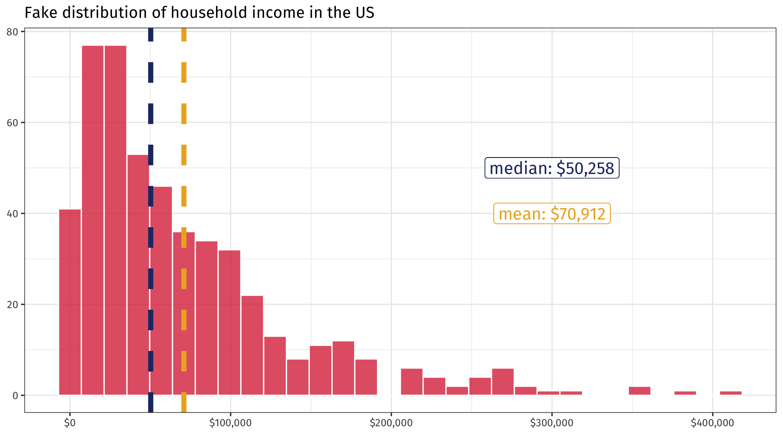
Mean vs. median

We almost always compare averages, but medians are helpful in some cases:

What’s happening here?

One more stat: variation

Another way to compare data is by how much a variable varies

Some distributions are very narrow, others are very wide

Narrow = observations are similar; wide = observations are not similar

Measuring variation: the standard deviation

The formula:

\[ s = \sqrt{\frac{1}{N-1} \sum_{i=1}^N (x_i - \overline{x})^2}\]

All the movement is here, the sum of the differences between each observation \(x_i\) and the average observation \(\overline{x}\)

\[\sum_{i=1}^N (x_i - \overline{x})^2\]

Variance intuition

Wide distribution

age	\(\overline{age}\)	\(\ age - \overline{age}\)	\(\ (age - \overline{age})^2 \)
87	55.3	31.7	1003.6
41	55.3	-14.3	205.1
23	55.3	-32.3	1044.6
45	55.3	-10.3	106.5
58	55.3	2.7	7.2

Narrow distribution

age	\(\overline{age}\)	\(\ age - \overline{age}\)	\(\ (age - \overline{age})^2 \)
48	49.9	-1.9	3.8
48	49.9	-1.9	3.8
52	49.9	2.1	4.2
48	49.9	-1.9	3.8
50	49.9	0.1	0.0

\[\sum_{i=1}^N (age_i - \overline{age})^2\]

The farther observations are from the mean, the larger the standard deviation

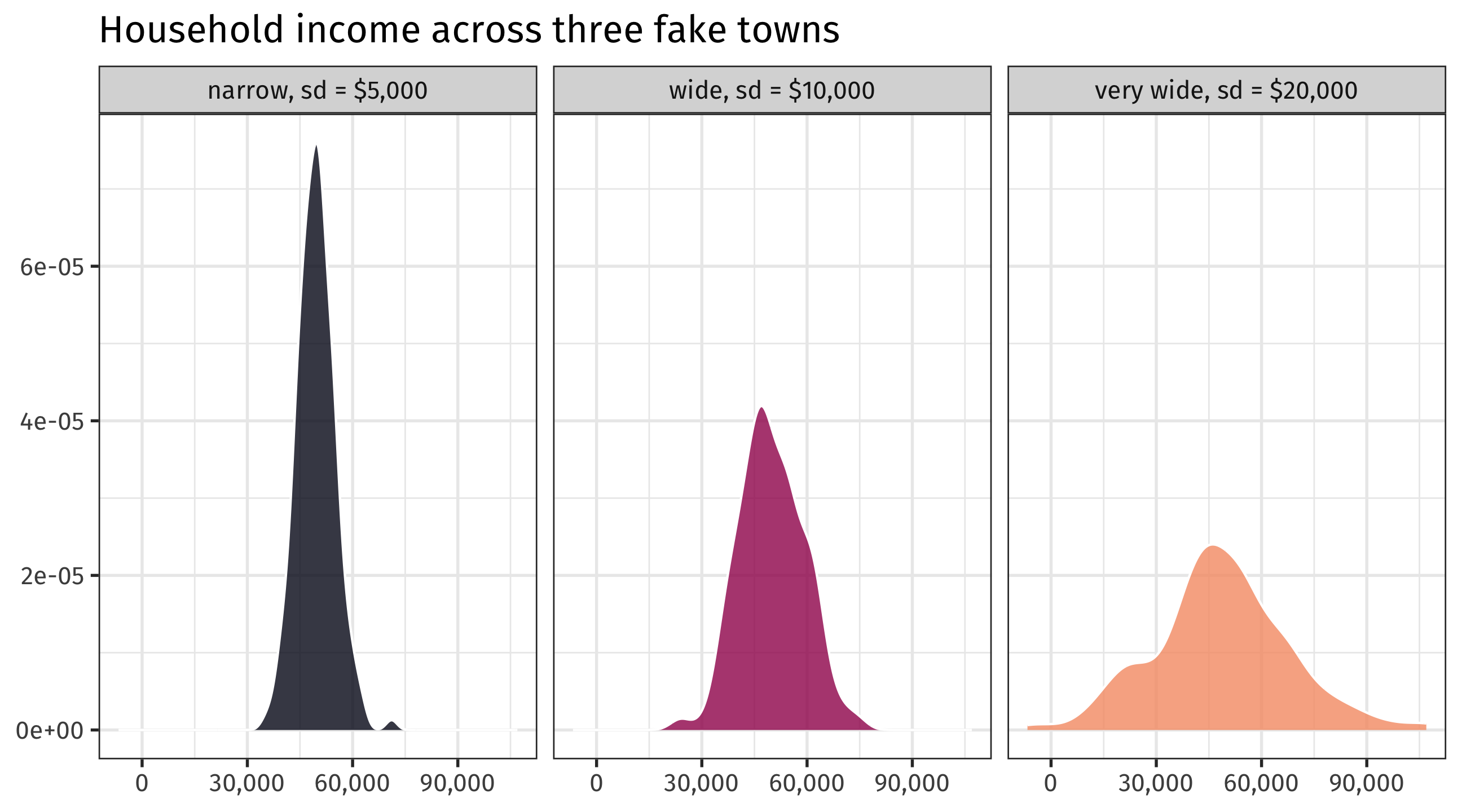
Measuring variation

Same average (~$50,000), different standard deviations

What could we measure with sd? Can we use standard deviation to measure equality?

Summarizing data in R

Summary statistics with summarize()

We can use summarize() to calculate things like the mean, median, etc.

Summarizing condenses data into statistics

Using summarize()

Say I want to know the average life expectancy in the world in 2007:

gapminder %>% 
  filter(year == 2007)

# A tibble: 142 × 6
   country     continent  year lifeExp       pop gdpPercap
   <fct>       <fct>     <int>   <dbl>     <int>     <dbl>
 1 Afghanistan Asia       2007    43.8  31889923      975.
 2 Albania     Europe     2007    76.4   3600523     5937.
 3 Algeria     Africa     2007    72.3  33333216     6223.
 4 Angola      Africa     2007    42.7  12420476     4797.
 5 Argentina   Americas   2007    75.3  40301927    12779.
 6 Australia   Oceania    2007    81.2  20434176    34435.
 7 Austria     Europe     2007    79.8   8199783    36126.
 8 Bahrain     Asia       2007    75.6    708573    29796.
 9 Bangladesh  Asia       2007    64.1 150448339     1391.
10 Belgium     Europe     2007    79.4  10392226    33693.
# ℹ 132 more rows

Using summarize()

gapminder %>% 
  filter(year == 2007) %>% 
  summarize()

# A tibble: 1 × 0

Using summarize()

gapminder %>% 
  filter(year == 2007) %>% 
  summarize(avg_life = mean(lifeExp))

# A tibble: 1 × 1
  avg_life
     <dbl>
1     67.0

Notice how the data has been summarized: only one row

Notice that I’ve named the summary statistic avg_life

Using summarize()

What if I also wanted to know the median life expectancy?

gapminder %>% 
  filter(year == 2007) %>% 
  summarize(avg_life = mean(lifeExp), 
            med_life = median(lifeExp)) 

# A tibble: 1 × 2
  avg_life med_life
     <dbl>    <dbl>
1     67.0     71.9

Notice! how similar this looks to mutate()

Using summarize()

What if I also wanted to know the min and max life expectancy?

gapminder %>% 
  filter(year == 2007) %>% 
  summarize(avg_life = mean(lifeExp), 
            med_life = median(lifeExp), 
            min_life = min(lifeExp), 
            max_life = max(lifeExp))

# A tibble: 1 × 4
  avg_life med_life min_life max_life
     <dbl>    <dbl>    <dbl>    <dbl>
1     67.0     71.9     39.6     82.6

Using summarize()

What if I also wanted to know the standard deviation of life expectancy?

gapminder %>% 
  filter(year == 2007) %>% 
  summarize(avg_life = mean(lifeExp), 
            med_life = median(lifeExp), 
            min_life = min(lifeExp), 
            max_life = max(lifeExp), 
            sd_life = sd(lifeExp))

# A tibble: 1 × 5
  avg_life med_life min_life max_life sd_life
     <dbl>    <dbl>    <dbl>    <dbl>   <dbl>
1     67.0     71.9     39.6     82.6    12.1

Using summarize()

gapminder %>% 
  filter(year == 2007) %>% 
  summarize(avg_life = mean(lifeExp), 
            med_life = median(lifeExp), 
            min_life = min(lifeExp), 
            max_life = max(lifeExp), 
            sd_life = sd(lifeExp)) 

summarize() is like mutate() in that you are creating new variables

So note that you have to name the new variables!

We can use summary functions in filter

which country had the lowest life expectancy in 2007?

gapminder %>% 
  filter(year == 2007) %>% 
  filter(lifeExp == min(lifeExp))

# A tibble: 1 × 6
  country   continent  year lifeExp     pop gdpPercap
  <fct>     <fct>     <int>   <dbl>   <int>     <dbl>
1 Swaziland Africa     2007    39.6 1133066     4513.

We can use summary functions in filter

which countries had above average GPD but below average health?

gapminder %>% 
  filter(year == 2007) %>% 
  filter(gdpPercap > mean(gdpPercap), lifeExp < mean(lifeExp))

# A tibble: 3 × 6
  country           continent  year lifeExp     pop gdpPercap
  <fct>             <fct>     <int>   <dbl>   <int>     <dbl>
1 Botswana          Africa     2007    50.7 1639131    12570.
2 Equatorial Guinea Africa     2007    51.6  551201    12154.
3 Gabon             Africa     2007    56.7 1454867    13206.

Woe unto us: missing data

In life, sometimes data is missing

respondent doesn’t answer a question, no one knows Afghanistan’s GDP in 1943, etc.

R represents missing data as NA

name	type1	type2	height_m	weight_kg
Lycanroc	rock	NA	NA	NA
Vulpix	fire	ice	NA	NA
Muk	poison	poison	NA	NA
Persian	normal	dark	NA	NA
Marowak	ground	fire	NA	NA
Graveler	rock	ground	NA	NA

Summarizing with missing data

If you try to summarize data that has missing values, R will return NA:

pokemon %>% 
  summarise(average_height = mean(height_m))

# A tibble: 1 × 1
  average_height
           <dbl>
1             NA

Note

Any math operation with NA will return NA (.e.g, 3 + NA = NA)

What to do?

There are whole classes on what to do with missing data (impute, simulate, model, etc.)

In this class we will tell R to ignore missing observations

We can do this by adding the na.rm = TRUE argument to summary

pokemon %>% 
  summarise(average_height = mean(height_m, na.rm = TRUE)) 

# A tibble: 1 × 1
  average_height
           <dbl>
1           1.16

Remember…

If you’re trying to calculate a summary statistic and keep getting NA…

99.99999% of the time you need to add na.rm = TRUE to your function!

pokemon %>% 
  summarise(average_height = mean(height_m, na.rm = TRUE)) 

# A tibble: 1 × 1
  average_height
           <dbl>
1           1.16

🚨 Your turn: 🚢 trade 🚢 🚨

Dataset from juanr on international trade:

Trade patterns around the world

country	year	imports	exports	gdp	pop	land_borders	sea_borders	min_cap_dist	sum_igos
United States of America	1946	5000	9775	2.479307e+12	138170640	2	1	0	44
United States of America	1947	5824	15369	2.430213e+12	139838676	2	1	0	47
United States of America	1948	7710	12470	2.494227e+12	143378709	2	1	0	52
United States of America	1949	7160	11920	2.466941e+12	146714635	2	1	0	57
United States of America	1950	9140	10220	2.562489e+12	149230105	2	1	0	59
United States of America	1951	11400	14920	2.729119e+12	150880698	2	1	0	60

🚨 Your turn: 🚢 trade 🚢 🚨

Using the trade dataset:

1. How has Inter-Governmental Organizations (IGOs) membership expanded over time? Calculate the median number of IGOs that countries belonged to in 1960. Repeat for 2010. About how much has IGO membership grown in 50 years?

2. What is having a sea border worth? Look only at countries that have at least one sea border in the year 2010. What is the average value of exports among these countries? Do the same for countries with no sea borders. About how much more do countries with sea borders export than countries without?

3. What was the country with the most exports in 1960? What about in 2012?

15:00

Relationships

summarize() lets us calculate statistics for the whole dataset

But what if we want to do this for different groups within the data?

This is at the heart of making comparisons

Variation in trade over time: the brutal way

How much do country imports vary for each country over time?

Tedious: filter() to calculate standard deviation of imports for each country

Starting with China

trade %>% 
  filter(country == "China") %>%  
  summarise(var_trade = sd(imports, na.rm = TRUE)) 

# A tibble: 1 × 1
  var_trade
      <dbl>
1   659178.

Variation in trade over time: the brutal way

I could go on to another country:

trade %>% 
  filter(country == "Algeria") %>%  
  summarise(var_trade = sd(imports, na.rm = TRUE)) 

# A tibble: 1 × 1
  var_trade
      <dbl>
1    14819.

Variation in trade over time: the brutal way

And so on for all countries… but this is brutally tedious

trade %>% 
  filter(country == "Nepal") %>%  
  summarise(var_trade = sd(imports, na.rm = TRUE)) 

# A tibble: 1 × 1
  var_trade
      <dbl>
1     2096.

Using group_by()

We can use group_by() in combination with summarize() to calculate some stat by another variable in the data:

trade %>% 
  group_by(country) %>%  
  summarise(var_trade = sd(imports, na.rm = TRUE)) 

# A tibble: 202 × 2
   country           var_trade
   <chr>                 <dbl>
 1 Afghanistan           2485.
 2 Albania               1754.
 3 Algeria              14819.
 4 Andorra                 NA 
 5 Angola                7584.
 6 Antigua & Barbuda       NA 
 7 Argentina            19530.
 8 Armenia               1575.
 9 Australia            72784.
10 Austria              58474.
# ℹ 192 more rows

Using group_by()

Like with anything else, we can store our results as a new object:

var_time = trade %>% 
  group_by(country) %>% 
  summarise(var_trade = sd(imports, na.rm = TRUE))

var_time

# A tibble: 202 × 2
   country           var_trade
   <chr>                 <dbl>
 1 Afghanistan           2485.
 2 Albania               1754.
 3 Algeria              14819.
 4 Andorra                 NA 
 5 Angola                7584.
 6 Antigua & Barbuda       NA 
 7 Argentina            19530.
 8 Armenia               1575.
 9 Australia            72784.
10 Austria              58474.
# ℹ 192 more rows

Variation in trade over time

And use our object to make plots:

What does this graph tell us?

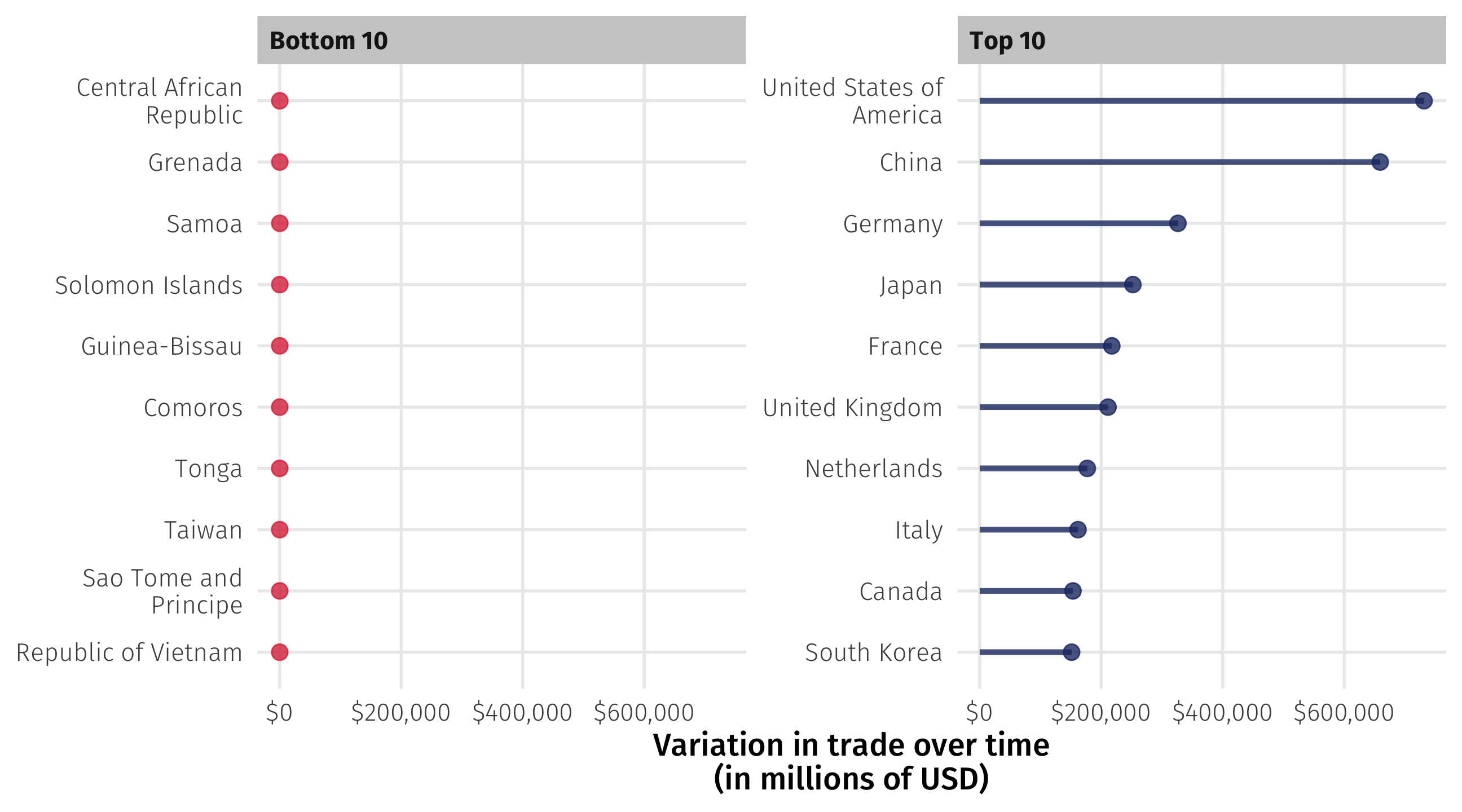
Using group_by()

We can even group_by() multiple variables 🤯

Average life expectancy per time:

gapminder %>%
  group_by(year) %>% 
  summarise(avg_life = mean(lifeExp))

# A tibble: 12 × 2
    year avg_life
   <int>    <dbl>
 1  1952     49.1
 2  1957     51.5
 3  1962     53.6
 4  1967     55.7
 5  1972     57.6
 6  1977     59.6
 7  1982     61.5
 8  1987     63.2
 9  1992     64.2
10  1997     65.0
11  2002     65.7
12  2007     67.0

Using group_by()

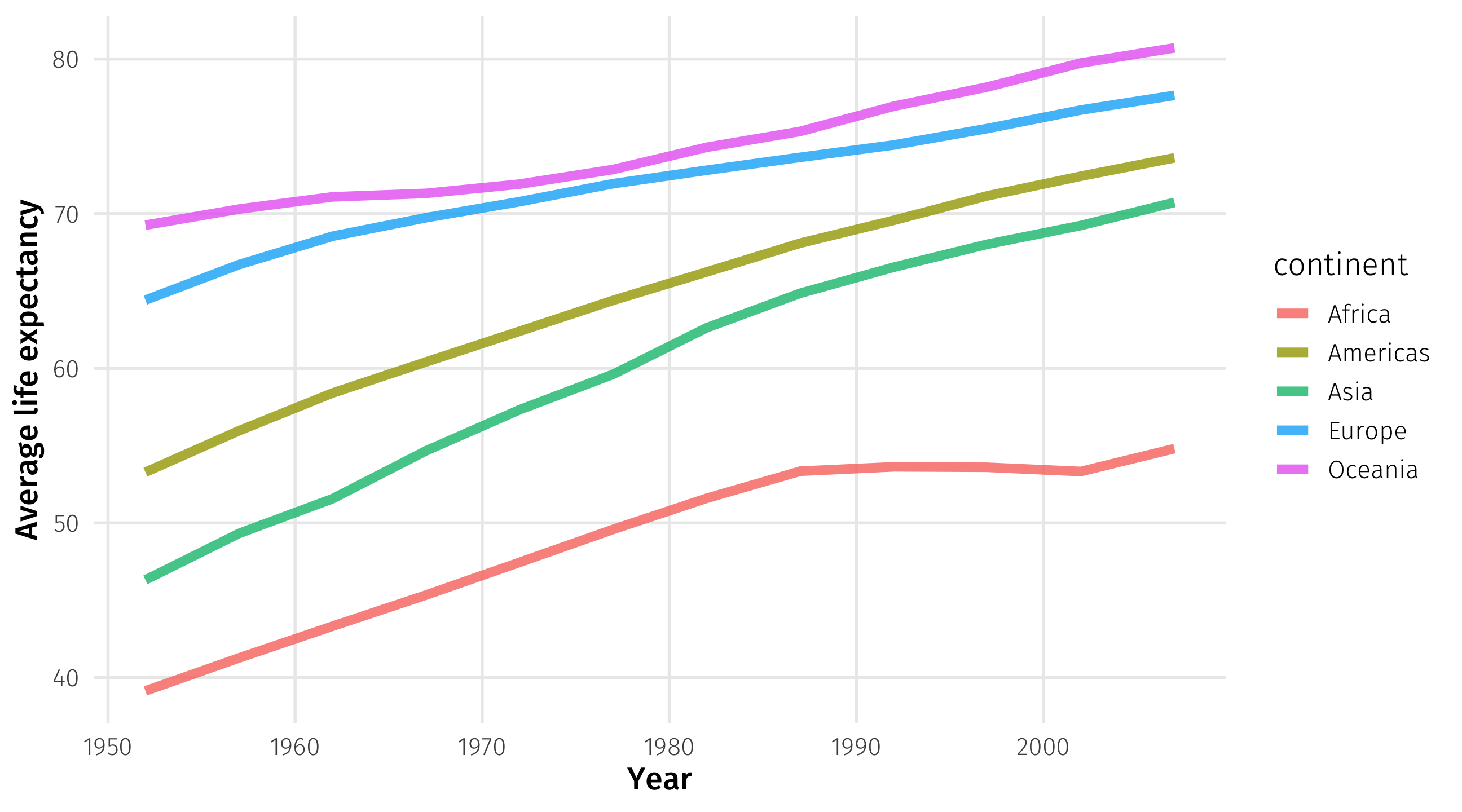
We can even group_by() multiple variables 🤯

Average life expectancy per year and continent:

gapminder %>%
  group_by(year, continent) %>% 
  summarise(avg_life = mean(lifeExp))

# A tibble: 60 × 3
# Groups:   year [12]
    year continent avg_life
   <int> <fct>        <dbl>
 1  1952 Africa        39.1
 2  1952 Americas      53.3
 3  1952 Asia          46.3
 4  1952 Europe        64.4
 5  1952 Oceania       69.3
 6  1957 Africa        41.3
 7  1957 Americas      56.0
 8  1957 Asia          49.3
 9  1957 Europe        66.7
10  1957 Oceania       70.3
# ℹ 50 more rows

Using group_by()

Store as object:

life_continent_year = gapminder %>% 
  group_by(year, continent) %>%
  summarise(avg_life = mean(lifeExp))

Make the plot

ggplot(life_continent_year, aes(x = year, y = avg_life, color = continent)) + 
  geom_line(size = 2, alpha = .8) + labs(x = "Year", y = "Average life expectancy")

🚨 Your turn: 🌡️ ugly prejudice 🌡️ 🚨

Researchers use feeling thermometers to measure how people feel about different groups

🌡 goes from zero (strong dislike) to 100 (strong like), with 50 as the neutral point

birth_year	sex	race	party_id	educ	ft_black	ft_white	ft_hisp	ft_asian	ft_muslim	ft_jew	ft_christ	ft_fem	ft_immig	ft_gays	ft_unions	ft_police	ft_altright	ft_evang	ft_dem	ft_rep
1931	Female	White	Democrat	4-year	51	50	79	50	50	50	50	99	95	50	80	76	1	50	88	21
1952	Female	White	Republican	2-year	98	90	95	100	61	100	98	65	96	82	62	95	50	96	86	96
1931	Male	White	Independent	High school graduate	87	90	91	88	49	25	50	74	77	77	100	78	0	2	91	20
1952	Male	White	Republican	4-year	90	85	90	96	80	91	94	25	91	71	20	94	50	70	22	83
1939	Female	White	Democrat	2-year	100	50	100	100	100	100	28	100	100	100	100	28	NA	NA	99	NA
1959	Female	Black	Democrat	Post-grad	98	70	99	100	100	100	100	73	100	54	80	24	4	53	53	4

🚨 Your turn: 🌡️ ugly prejudice 🌡️ 🚨

Using the therm dataset:

1. Calculate average 🌡 towards two groups of your choosing, broken down by one respondent characteristic. Make sense of the finding.

2. Calculate average 🌡 towards two groups of your choosing, broken down by two (🤯🤯🤯) respondent characteristics. Make sense of the finding.

15:00

How Americans feel about different groups